
doing topology with types
Post Metadata
This blog post was written by Bryan Lu, a rising third-year graduate student in UW’s mathematics department studying algebraic combinatorics. Once upon a time, they caught the formal methods bug from their undergraduate studies at Cornell University, and learned a significant amount about proof assistants, programming languages, and compilers. As of recently, they have continued to scratch this particular interest by hanging out with the PLSE group in various capacities, and are excited to continue lurking around the lab.
Most people who’ve worked with a programming language probably have some sense of what types are – they’re these abstract labels that organize the values that we work with. Before reading on, though, I’d like you to take a moment to think about how to interpret a type as an object – what mental construction do you think of when you think of a type?
Got an answer in mind? Great!
One mental construction you likely conjured to describe a type is the (mathematical) set. This makes sense for most data types, like the integers, the natural numbers, or the booleans. This is a pretty reasonable construction!
If you’re familiar with dependent types and the Curry-Howard correspondence, you might remember that types correspond to propositions. This is super important for proof assistants like Rocq or Lean, since now elements of a type correspond to evidence for that proposition. This allows one to write down programs which “prove” the theorem given by the program’s type. However, this interpretation is a little clunky for data types – for instance, an element n : nat of the natural numbers is now interpreted as evidence that some natural number \(n\) exists. But this is a little silly, since we’d like to think of elements that have type nat as numbers proper, not just “evidence”. In my opinion, both of these interpretations of types are reasonable, but aren’t super elegant taken together. This is a bit of a problem, since it would be nice to have a single abstraction that models the use cases of types as both propositions and sets!
From the point of view of homotopy type theory, a better mental construction that unifies these two interpretations of types is a visual one describing types as topological spaces. Topological spaces are the fancy mathematical word that we use to describe shapes in the “squishy” sense – that is, we consider two topological spaces the same if one can continuously deform one to get the other. This notion of a “squishy” space is the construction we’ll use to describe our types, with elements of that type being the points of that space. We’ll see how the types we’re used to working with can be interpreted as spaces, and how this more general framework allows us to construct stranger types that model shapes that we are familiar with.
re-introducing: inductive types
We can generally interpret the data types that we work with as inductive types. To define an inductive type, we need to know how to construct elements of that type and how to process an element of that type in a function. The canonical example is the type of the natural numbers, here given in Agda syntax:
data nat : Type where
  zero-nat : nat
  succ-nat : nat -> nat
Here we have two constructors, zero-nat representing the number \(0\) in the natural numbers, and the successor function succ-nat giving the successor of any previously existing natural number. For instance, succ-nat zero-nat represents the successor of \(0\), which is \(1\). Therefore, from here on out, we’ll abuse notation and write 0 for zero-nat, and use all other natural numbers to describe succ-nat applied to zero-nat that many times (e.g. by 1, we mean succ-nat zero-nat). We’ll also use S as shorthand for succ-nat.
The natural numbers come with an induction principle, describing how to construct recursive functions with domain nat. Here is its type declaration:
nat-elim : (P : nat -> Type)
  -> P zero-nat
  -> ((k : nat) -> P k -> P (succ-nat k))
  -> ((n : nat) -> P n)
The function nat-elim (so named as it describes the “elimination rule” for the natural numbers) allows us to define functions on the natural numbers recursively. Notice that nat-elim has a type signature that really looks like the principle of mathematical induction. Recall induction says that given a family of propositions \(P(n)\) indexed by natural numbers \(n \in \mathbb N\), a proof of \(P(0)\) (the base case), and a proof that for any \(k \in \mathbb N\), a proof of \(P(k)\) implies a proof of \(P(k+1)\) (the inductive case), one can show \(P(n)\) for all \(n \in \mathbb N\). Taking Type as a synonym for “proposition” by Curry-Howard, in nat-elim, we should correspondingly think of the argument of type P zero-nat as the base case and the function of type (k : nat) -> P k -> P (succ-nat k) as the inductive case.
All inductive types come with an induction principle. As a good exercise, consider the type of the integers:
data int : Type where
  pos-int : nat -> int
  zero-int : int
  neg-int : nat -> int
where we zero-index our positive and negative integers, so that pos-int 0 represents \(1\) and neg-int 0 represents \(-1\). Can you write down the corresponding induction principle for int?
equality is the path forward!
A more subtle example of an inductive type is the equality type \(\equiv\) for any type \(A\). Here, for any element \(a : A\), we consider the type of equalities
data _≡_ {A : Type} (a : A) : A -> Type where
  refl : a ≡ a
infix 0 _≡_
(To avoid confusion with the usual \(=\), we’ll use \(\equiv\) for the equality type here.)
The equality type has a single constructor, refl, which describes the fact that for any element \(a\) of type \(A\), \(a\) is equal to itself. Mathematically, we know this as the property that equality is reflexive, hence refl. We call this type “equalities based at \(a\).”
The induction principle for this equality type has a special name, often called (based) path induction:
≡-elim : {A : Type} -> (x : A)
  -> (P : (y : A) -> x ≡ y -> Type)
  -> (P x refl)
  -> (y : A) -> (p : x ≡ y) -> P y p
This principle essentially says that for some fixed \(x : A\), given a \(y : A\) and evidence that \(x \equiv y\), to prove a proposition \(P\) that might depend on both \(x\) and \(y\), it suffices to prove \(P\) with all instances of \(y\) replaced by \(x\) (which we denote \(P[x/y]\)). This should hopefully feel fairly intuitive! Type-theoretically, since the equality type based at \(x\) has a single constructor for a given inductive type \(A\), to process an equality based at \(x\), it suffices to consider when that equality is of two elements that are exactly identical.
As an application, we can use it to prove equality is both symmetric and transitive:
-- Type declaration of ≡-sym:
≡-sym : {A : Type} (x y : A) -> x ≡ y -> y ≡ x
-- Proof of ≡-sym:
≡-sym x y p = ≡-elim x (λ z _ -> z ≡ x) refl y p

-- Type declaration of ≡-trans:
≡-trans : {A : Type} (x y z : A) -> x ≡ y -> y ≡ z -> x ≡ z
-- Proof of ≡-trans:
≡-trans x y z p q = ≡-elim y (λ w _ -> x ≡ w) p z q
What are these two proofs saying?
- For
≡-sym, since \(x \equiv y\), to prove \(y \equiv x\), it suffices to prove \((y \equiv x)[x/y] = (x \equiv x)\) in the case where we substitute \(x\) for \(y\) everywhere. In particular, we need to prove \(x \equiv x\), which is just reflexivity. - For
≡-trans, we want to prove \(x \equiv z\). Since \(y \equiv z\), it suffices then to prove \((x \equiv z)[y/z] = (x \equiv y)\). But we have evidence for this already.
Let’s break down what’s happening here type-theoretically:
- For
≡-sym, we want to use the equalityp : x ≡ y, so we want to use the induction principle for the type of equalities based at \(x\). The predicatePneeds to takeyandpand turn them into a term of typey ≡ x, soPmust be the function type(λ z _ -> z ≡ x). Path induction tells us it suffices to give a term of typeP x reflwhich is actually the typex ≡ x. But there’s an obvious term of this type – namely,refl. - For
≡-trans, we want to use the equalityq : y ≡ z, so we want to use the induction principle for the type of equalities based at \(y\). The predicatePneeds to takezandqand turn them into a term of typex ≡ z, soPmust be the function type(λ w _ -> x ≡ w). Path induction tells us it suffices to give a term of typeP y reflwhich is actually the typex ≡ y. But we already have a term of this type in our hypotheses.
So why is this principle called “path induction”? Here’s the critical correspondence that makes this analogy work:
For terms \(x, y : A\), a term of the equality type \(x \equiv y\) corresponds to a path in \(A\) from \(x\) to \(y\).
From this point of view, given a point \(x\) in the space \(A\), to prove a statement about a point \(y\) connected to \(x\) by a path, we can “follow the path” from \(y\) back to \(x\). Then, a proof that the statement holds at \(x\) can be “transported” along the path to \(y\).
From this point of view, the lemma ≡-sym tells you that if you have a path from a point \(x\) to a point \(y\), then you have a path in the opposite direction from \(y\) to \(x\). Similarly, ≡-trans tells you that you can concatenate a path from \(x\) to \(y\) and a path from \(y\) to \(z\) into a path from \(x\) to \(z\).
Those acquainted with some basic algebraic topology might recognize these lemmas as the start of the group laws for the concatenation operation! In particular, ≡-sym precisely allows us to define the inverse of a path (which we denote by !), and ≡-trans allows us to define concatenation of paths (which we denote by ∙):
! : {A : Type} {x y : A} -> x ≡ y -> y ≡ x
! {A} {x} {y} = ≡-sym {A} x y

_∙_ : {A : Type} {x y z : A} → x ≡ y → y ≡ z → x ≡ z
_∙_ {A} {x} {y} {z} = ≡-trans {A} x y z
infixl 7 _∙_
As an exercise with path induction, one can try to show that applying a function \(f : A \to B\) to a path \(x \equiv y\) behaves as expected1. This property is usually referred to as congruence:
cong : {A B : Type} (f : A -> B) {x y : A}
  -> x ≡ y -> f x ≡ f y
cong = ?
This interpretation of types as spaces places special emphasis on types \(A\) where in the space interpretation, every point is connected by a path to some center point \(c : A\). Such types are called contractible, with \(c\) being the center of contraction. These types end up being generally boring – such types are exactly the ones isomorphic (in some sense) to the unit type True, with one trivial constructor, intro. As we’ll see later, though, contractible types are what one uses to distinguish between types that are propositions and types that are sets.
There is a large world of non-contractible types that are inhabited – a couple easy examples are the boolean type bool with two constructors true and false, or the natural numbers nat with a countable number of unequal terms. However, both these examples are non-contractible because they have a discrete collection of multiple distinct terms of that type. If we allow ourselves to think topologically, though, we can construct some fairly nontrivial types that will visually be non-contractible, but only have very few terms of that type.
what if we went higher?
It’s not strictly necessary that the constructors of our type only tell us how to get elements of that type in homotopy type theory. One of the main extensions to the theory is allowing ourselves to also have type constructors for the equality types of terms, which gives us higher inductive types. For example:
postulate
  S1 : Type
  pt : S1
  loop : pt ≡ pt
Normally, Agda is not very happy about this definition especially since we have a second constructor for the equality type pt ≡ pt in S1 that is not refl! We get around this here by using postulate to tell Agda to just trust us on this one, but there are certain flavors of Agda that will allow us to establish such constructors without this hack2. Visually, this type looks like the following space:
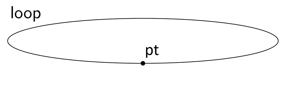
Technically, I’ve omitted a loop refl connecting pt to itself – we usually interpret the path corresponding to refl as the constant path at pt, up to homotopy. What this loosely means is that refl is also the interpretation of any path that can be continuously deformed to the constant path. The loop constructor for S1, by the injectivity of constructors, cannot be equal to refl, so this is a path from pt to pt that cannot be shrunk down to the constant path at pt. Strangely, though, even though visually it looks like there are many unmarked points on this path loop from pt to itself, the only term of the type S1 that we have is pt, by our constructors. In particular, any term of type S1 will be equal to pt, but two given proofs of that fact pt ≡ pt may not necessarily be equal! Higher inductive types therefore are a way of constructing types that fail to satisfy the principle of proof irrelevance, thinking of pt as a proof of S1 in this instance.
Visually, though, S1 looks like a circle! Mathematicians call the circle \(S^1\) – hence the naming of this type (which folks sometimes informally call the circle type). Writing down the correct induction principle3 for the circle now starts to get complicated, and we have to now postulate it:
postulate
  S1-rec : {X : Type} (x : X) (p : x ≡ x) → S1 → X
  S1-rec-base : {X : Type} (x : X) (p : x ≡ x)
                  → (S1-rec {X} x p pt) ≡ x
{-# REWRITE S1-rec-base #-}
postulate
  S1-rec-loop : {X : Type} (x : X) (p : x ≡ x)
              → (cong (S1-rec x p) loop) ≡ p
We’re using a little bit of Agda wizardry here with the line {-# REWRITE S1-rec-base #-} so that S1-rec-loop looks like a well-formed type – it’s safe to ignore, for our purposes. What’s more important is that this induction principle tells us how to define functions that use a value of type S1 and produce a value of type X. In particular, the hypotheses tell us that we need an x : X and a path p : x ≡ x from x back to itself to define this map. S1-rec-base tells us that x needs to be the image of the pt : S1 under the function defined by S1-rec, and (after unfolding some equalities, using the equality given to us by S1-rec-base) we require that the image of the loop constructor, loop : pt ≡ pt, must be the path p : x ≡ x. Visually, we can think of the proposition S1-rec as saying that a map from the circle \(S^1 \to X\) is given by a choice of point \(x \in X\) and loop \(p\) joining \(x\) to itself, which embeds the circle \(S^1\) into the space \(X\).
Here’s a more complicated type:
postulate
  T : Type
  pt : T
  a : pt ≡ pt
  b : pt ≡ pt
  sq : a ∙ b ≡ b ∙ a
Again, we have two nontrivial constructors a and b for the equality type pt ≡ pt, corresponding to two loops in our space that cannot be contracted down to the constant path at pt, refl. We also have a constructor for the equality type _≡_ {pt ≡ pt} on paths. This corresponds to a path sq between the composite paths a ∙ b and b ∙ a, which we can think of as a square that fills in a region bounded by these two paths. We can represent the space that this makes in the following way:
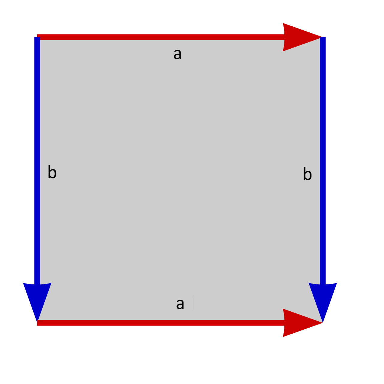
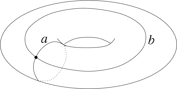
If we take this square given to us by this path-between-paths and glue the opposite sides a and b where they match, we see that this type models a torus!
A similar trick will allow us to construct types that represent arbitrary surfaces. As an exercise, see if you can work out what these types should be, topologically (their names give them away, if you recognize them):
postulate
  S2 : Type
  base : S2
  surf : _≡_ {base ≡ base} refl refl
postulate
  RP2 : Type
  u : RP2
  v : RP2
  x : u ≡ v
  y : v ≡ u
  cell : x ∙ y ≡ (! y) ∙ (! x)
postulate
  SS1 : Type
  N : SS1
  S : SS1
  merid : S1 -> (N ≡ S)
(two of these will be the same, and none are contractible!4)
In general, any topological space that can be built from gluing together points, paths, surfaces, etc. can be constructed as a higher inductive type. (Mathematicians generally refer to such spaces as CW-complexes.) This allows one to use type theory to directly prove topological statements! As a gateway into what this might look like – one could try to prove, for instance, that the type of loops on the circle is isomorphic to the integers. Folks familiar with algebraic topology would recognize this as saying \(\pi_1(S^1) \cong \mathbb Z\). Doing this in types requires the univalence axiom, which is the other innovation of homotopy type theory. Loosely, this axiom allows one to take two types that are “equivalent” and generate an equality of those types, which will end up being necessary to construct the maps back and forth between the type of loops on S1 and the integers.
what happens to propositions and sets?
Let’s go back to our motivating conflict of interest. What kinds of spaces should propositions look like? In first-order logic, we can think of propositions as either being true or false. If the proposition is true, we don’t really have a way of distinguishing between them in the logic, so we treat all of the proofs of that proposition as the same. From the space point of view, the type corresponding to a proposition should either be empty or any two terms of that type should be equal, i.e. they are either contractible or completely uninhabited. In particular, if a proposition \(P\) has a proof \(p : P\), then all proofs of that proposition are equal – we call this proof irrelevance in our proof assistants. It turns out that this is equivalent to saying that the equality types for elements of a proposition are contractible.
What about for sets? Here, the points of a set can be arbitrary, so the constraints we want won’t have to do with the terms of the type themselves. Notably, for a set, determining whether an element is in the set or not is a proposition. This means that checking the equality of elements in a set must also be a proposition, and in particular this is the definition that we take in homotopy type theory to characterize sets.
In general, we can start building a hierarchy of types called \(n\)-types, with contractible types at the base. (Sometimes the levels of this hierarchy are referred to as h-levels, or truncation levels.) The hierarchy begins as follows with (the strange choice) \(n = -2\), where the equality types of \(n+1\)-types are \(n\)-types:
| h-level | name of type |
|---|---|
| -2 | contractible types |
| -1 | propositions |
| 0 | sets |
| 1 | groupoids |
| 2 | ??? |
| … | … |
The reason for the strange numbering is so that it lines up with the mathematical notion of homotopy \(n\)-types in homotopy theory. For those familiar, a space has homotopy \(n\)-type if the homotopy groups \(\pi_k(X)\) vanish for all \(k > n\). Discrete sets with no nontrivial topological structure, for instance, have no nontrivial homotopy groups \(\pi_k\) for any \(k > 0\). It turns out that under the types-as-spaces interpretation, with this numbering, the h-level of the type and the homotopy \(n\)-type of the corresponding space coincide! This makes, for example, the circle type S1 above a 1-type, and the type S2 above an \(\infty\)-type (as with most types that give nontrivial spaces).
At any rate, this shows how the homotopy type theory interpretation of types as spaces allows us to reason about and distinguish our types as being propositions, sets, or something else entirely! For further reading about this extension of dependent type theory, consider checking out The HoTT Book or Introduction to Homotopy Type Theory (Rijke, ‘22) and/or playing with the Agda proof assistant!
endnotes
-
by path induction, we can treat our path argument as
refl, at which point our definition iscong f refl = refl↩ -
There are ways around these postulates – a flavor of Agda called cubical Agda allows one to work with these ↩
-
technically, this is a recursion principle, not an induction principle – notice that we don’t have full dependence in \(X\) here ↩
-
the first and third are both the 2-sphere \(S^2\), and the second is the real projective plane \(\mathbb R P^2\) ↩