Chaotic Dynamical Systems Using JAX

In this blog post, I will focus on how JAX works (and where it does not work) for dynamical systems.

Dynamical systems describe how a system changes over time according to fixed rules. JAX seems like a good fit because it makes numerical code easier to compile, parallelize, and differentiate. But what happens if a dynamical system is chaotic?

1. What is JAX and How to Think in JAX

The JAX documentation describes JAX as a library for array-oriented numerical computation, à la NumPy, with automatic differentiation and JIT compilation for high-performance machine learning research. Historically, JAX stood for “Just After eXecution” because early versions monitored one Python execution before compilation. People have also used informal backronyms such as “Just-in-time compilation, Autodiff, and XLA” and “Just Another XLA” over time. Today, JAX is simply JAX.

One big advantage of JAX is that it shares a similar API with NumPy, while also being able to run on accelerators such as GPUs and TPUs. For example, you can often replace numpy with jax.numpy:

import numpy as np

np_array = np.array([1, 2, 3])
print("np_array", np_array, type(np_array))

import jax.numpy as jnp

jnp_array = jnp.array([1, 2, 3])
print("jnp_array", jnp_array, type(jnp_array))

Output:

np_array [1 2 3] <class 'numpy.ndarray'>
jnp_array [1 2 3] <class 'jaxlib._jax.ArrayImpl'>

Even though JAX appears very similar to NumPy, it is not just a drop-in replacement for NumPy. As Alex McKinney explains in On Learning JAX, JAX is less about manipulating arrays operation by operation and more about defining a computational graph that the compiler can optimize.

Here are a few general rules for writing JAX code:

• JAX transformation and compilation are designed to work only on Python functions that are functionally pure.

• JAX arrays are immutable. If we continue the previous example:

  To modify a NumPy array, we can simply assign the value to the index:

  np_array[0] = 4
  print("np_array", np_array)
  

  Output:

  np_array [4 2 3]
  

  However, jnp_array[0] = 4 gives us a TypeError: JAX arrays are immutable and do not support in-place item assignment. Instead of x[idx] = y, use x = x.at[idx].set(y) or another .at[] method: https://docs.jax.dev/en/latest/_autosummary/jax.numpy.ndarray.at.html

  new_jnp_array = jnp_array.at[0].set(4)
  print("new_jnp_array", new_jnp_array)
  print("jnp_array", jnp_array)
  

  Output:

  new_jnp_array [4 2 3]
  jnp_array [1 2 3]
  

  Updates return a new array, and the original array is not modified.

• JAX avoids implicit global random state, and instead tracks state explicitly via a random key:

  key = jax.random.key(42)
  print(key)
  

  Output:

  Array((), dtype=key<fry>) overlaying:
  [ 0 42]
  

  To convert one key into several independent (in the pseudorandomness sense) keys:

  key, subkey = jax.random.split(key)
  

Configuration

For all the numerical experiments in this post, I use the following configuration:

Install and import JAX

!pip install jax

import jax
import jax.numpy as jnp
print("Using JAX", jax.__version__)

Output:

Using JAX 0.9.2

Use all available CPU devices

import os

num_cpu_devices = os.cpu_count() or 1
jax.config.update("jax_num_cpu_devices", num_cpu_devices)

print("Device count:", jax.device_count())
print("Devices:", jax.devices())

Output:

Device count: 10
Devices: [CpuDevice(id=0), CpuDevice(id=1), CpuDevice(id=2), CpuDevice(id=3), CpuDevice(id=4), CpuDevice(id=5), CpuDevice(id=6), CpuDevice(id=7), CpuDevice(id=8), CpuDevice(id=9)]

Enable 64-bit floating point arithmetic

jax.config.update("jax_enable_x64", True)
print("JAX_ENABLE_X64:", jax.config.read("jax_enable_x64"))

Output:

JAX_ENABLE_X64: True

2. Dynamical Systems

In mathematics, physics, engineering and systems theory, a dynamical system is the description of how a system evolves in time.

A dynamical system can be written as a tuple \((T, \mathcal{M}, \Phi)\), where

• \(T\) is the time set, usually \(\mathbb{Z}\) or \(\mathbb{R}\)
• \(\mathcal{M}\) is the state space, which is the set of all possible states \(x\).
• \(\Phi: T \times \mathcal{M} \to \mathcal{M}\) is an evolution operator, where \(\Phi(t, x)\) is the state reached by evolving state \(x\) for time \(t\). It satisfies \(\Phi(0, x) = x\) and \(\Phi(t + s, x) = \Phi(t, \Phi(s, x))\) for all \(t, s \in T\) and states \(x \in \mathcal{M}\).

Two common forms are:

• Discrete-time system: \(x_{n+1} = F(x_n)\)

  The function \(F\) takes the current state \(x_n\) and produces the state \(x_{n+1}\) at the next time step.

• Continuous-time system, also called a flow, is generated by the ODE

  \[\frac{d\mathbf{x}}{dt} = \mathbf{f}(\mathbf{x}; s), \qquad \mathbf{x}(0) = \mathbf{x}_0.\]

  In this equation, the state \(\mathbf{x}\) changes continuously over time. The vector field \(\mathbf{f}\) gives its instantaneous rate of change at each state, starting from the initial state \(\mathbf{x}_0\).

  The discrete-time map induced by the flow over a time step \(\Delta t\) is

  \[\varphi(\mathbf{x}) := \Phi^{\Delta t}(\mathbf{x}), \qquad \mathbf{x}_{k+1} = \varphi(\mathbf{x}_k).\]

Here \(x_n\) is the state at time step \(n\), \(F\) is a discrete-time map, \(t\) is continuous time, \(\mathbf{f}\) is the continuous-time vector field, and \(\varphi = \Phi^{\Delta t}\) is the discrete-time map induced by the flow. A trajectory is a sequence of states ordered by time.

Usually in dynamical systems, we care about:

• Predicting future states
• Determining long-term behavior, such as equilibrium, periodicity, or chaos
• Computing statistical properties
• Measuring sensitivity to initial conditions or parameters
• Controlling or optimizing the system’s behavior

Chaos

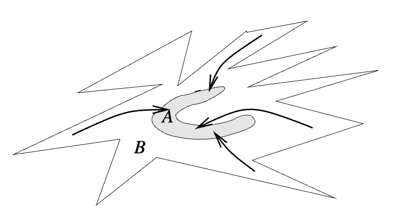
An attractor is a set of states toward which a system tends to evolve.

On an aperiodic, or non-periodic, attractor, small differences in initial conditions on the attractor lead at later times to large differences, still on the attractor.

Two effects happen at the same time:

• Attraction, such that the trajectories converge.
• Sensitivity to initial conditions, such that nearby trajectories diverge along unstable directions, often at an exponential rate.

Trajectories converge to the attractor, but diverge on the attractor.

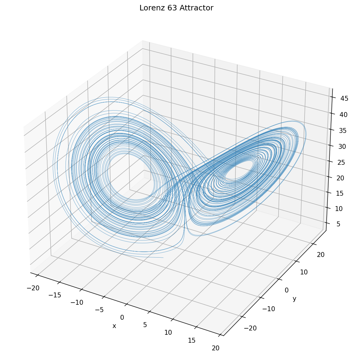
Lorenz 63

Lorenz 63, developed by Edward Lorenz, is a classic example of a system that can exhibit chaotic behavior. It is defined by the following equations:

where:

• Prandtl number \(\sigma = 10.0\)
• Parameter relates to the physical dimensions of the fluid layer itself: \(\beta = 8.0 / 3.0\)
• Rayleigh number \(\rho = 28.0\)

More broadly, studying a dynamical system can involve several goals:

• Predicting future states
• Determining long-term behavior, such as equilibrium, periodicity, or chaos
• Computing statistical properties
• Measuring sensitivity to initial conditions or parameters
• Controlling or optimizing the system’s behavior

3. Timestepping

Recall that the one-step map is \(\mathbf{x}_{k+1} = \varphi(\mathbf{x}_k)\). We numerically approximate this map using the fourth-order Runge-Kutta (RK4) method with a fixed time step size \(\Delta t\):

To build a trajectory, we need to apply this one-step update rule many times. In JAX, jax.lax.scan is the appropriate tool for this kind of repeated recurrence.

def integrate(system, state, params, T_total):
    num_steps = int(T_total / system.dt)

    # carry represents the current state x_k
    def scan_step(carry, _):
        next_state = rk4_step(system, carry, params) # applies the one step map to get x_{k+1}
        return next_state, next_state
    # The first next_state becomes the carry for the next iteration, so the next scan step receives x_{k+1}.
    # The second next_state is saved into the output trajectory.

    final_state, trajectory = jax.lax.scan(scan_step, state, None, length=num_steps)

    return final_state, trajectory

Therefore, after \(N = T_{\text{total}} / \Delta t\) iterations, scan returns the final state \(x_N\) and the full trajectory \((x_1, \ldots, x_N)\).

Conceptually, jax.lax.scan is similar to this Python loop:

carry = init
ys = []
for x in xs:
    carry, y = f(carry, x)
    ys.append(y)
return carry, np.stack(ys)

Then use jax.jit to compile the whole time integration routine into optimized XLA code:

jit_integrate = jax.jit(integrate,static_argnames=("system", "T_total"))

One key takeaway is that jax.jit is very powerful and should be used around the largest repeated computation that has a stable shape and control-flow structure.

Here system and T_total are static. system is a python object that is not an array. And num_steps= int(T_total / system.dt), which is the length of jax.lax.scan, must be known when JAX compiles the function, so T_total cannot be a dynamical value. If they change, JAX may need to recompile.

system = Lorenz63()
params = Lorenz63Params()
T_total = 100.0
state0 = system.init_state(jax.random.PRNGKey(2))

print("`integrate` time")
%time integrate(system, state0, params, T_total)[1].block_until_ready()

print("`jit_integrate` first call")
jit_integrate = jax.jit(integrate, static_argnames=("system", "T_total"))
%time jit_integrate(system, state0, params, T_total)[1].block_until_ready()

print("`jit_integrate` time")
%timeit jit_integrate(system, state0, params, T_total)[1].block_until_ready()

During this first call, the shapes of the input arrays will be used to trace out a computational graph, stepping through the function with the Python interpreter and executing the operations one-by-one, recording in the graph what happens. This intermediate representation can be given to XLA and subsequently compiled, optimised, and cached. This cache will be retrieved if the same function is called with the same input array shapes and dtype, skipping the tracing and compilation process and calling the heavily optimised, precompiled binary blob directly.

It is also important to use block_until_ready() for timing/benchmarking. JAX often dispatches work asynchronously, so it does not wait for the operation to complete before returning control to Python. Calling block_until_ready() forces the timing cell to wait for the numerical computation to complete.

Output:

`integrate` time
CPU times: user 89 ms, sys: 130 ms, total: 219 ms
Wall time: 346 ms

`jit_integrate` first call
CPU times: user 70.2 ms, sys: 11.7 ms, total: 81.9 ms
Wall time: 71.7 ms

`jit_integrate` time
853 us +/- 58.6 us per loop (mean +/- std. dev. of 7 runs, 1,000 loops each)

Like expected, the first jit_integrate call will take much longer than the subsequent calls. It is important to exclude the first call from any benchmarking for this reason. We also see that even for this simple example the compiled version of the function executes far quicker than the original function.

4. Observables

In chaotic systems, there is the butterfly effect, which describes how small changes to a complex system’s initial conditions can produce large differences in its later states. Because of this, accurate pointwise prediction of a single long-time trajectory is usually not possible. However, one can often compute stable statistical quantities associated with the dynamics, which, for example, can be long-time average observables.

Let \(\varphi: \mathcal{M} \to \mathcal{M}\) be the discrete-time one-step map on the state space \(\mathcal{M}\). Given an initial condition \(\mathbf{x}_0 \in \mathcal{M}\), the trajectory is

An observable is a real-valued function on state space:

Assume that the dynamical system admits a natural invariant probability measure \(\mu\) on the attractor, and that \(\mu\) is ergodic. Intuitively, ergodic means that a typical sufficiently long trajectory samples the system according to this invariant probability distribution. Birkhoff’s ergodic theorem then implies that, for \(\mu\)-almost every initial condition \(\mathbf{x}_0\), the time average

exists and satisfies

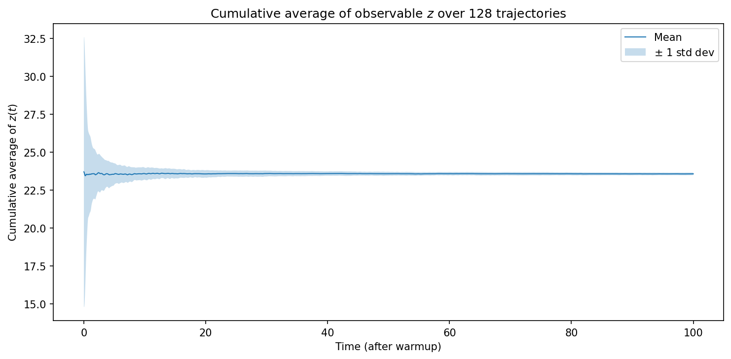
In the following example, target statistical quantity is the long-time average of an observable. We can examine the quantity at two levels: the cumulative time average along each trajectory and the mean and standard deviation of the final time averages across many trajectories.

For Lorenz 63, let the observable be the value of \(z\) coordinate:

Cumulative time average along one trajectory.

After a warmup time of \(T=100\), I compute the cumulative time average of the \(z\) coordinate for another \(T=100\) with timestep \(\Delta t = 0.005\):

def observable_z(state):
    return state[2]

jax.vmap turns a function that acts on one input into a function that acts on a batch of inputs. By default, in_axes=0, so vmap maps over the leading axis of the input array. Here, observable_fn computes the observable for one state, and vmap applies it to every state in the trajectory at once:

obs = jax.vmap(observable_fn)(traj[steps_warmup:])

The cumulative time average along this trajectory is computed by

jnp.cumsum(obs) / jnp.arange(1, obs.shape[0] + 1)

and the (m)-th entry of this array is \(\frac{1}{m} \sum_{k=0}^{m-1} S(\mathbf{x}_{k_0+k})\) , where \(m = 1, 2, \ldots, \texttt{steps\_main}\)

Mean and standard deviation across trajectories.

The second use of jax.vmap is:

keys = jax.random.split(key, batch_size)
obs_batch = jax.vmap(one_traj)(keys)

Here, one_traj computes the cumulative time average for one initial condition, while jax.vmap(one_traj)(keys) repeats this computation for trajectories with randomly sampled initial conditions. The resulting batch has

where the mean estimates the invariant-measure average of \(z\) and the standard deviation measures variation among the finite-time averages.

5. Autodiff

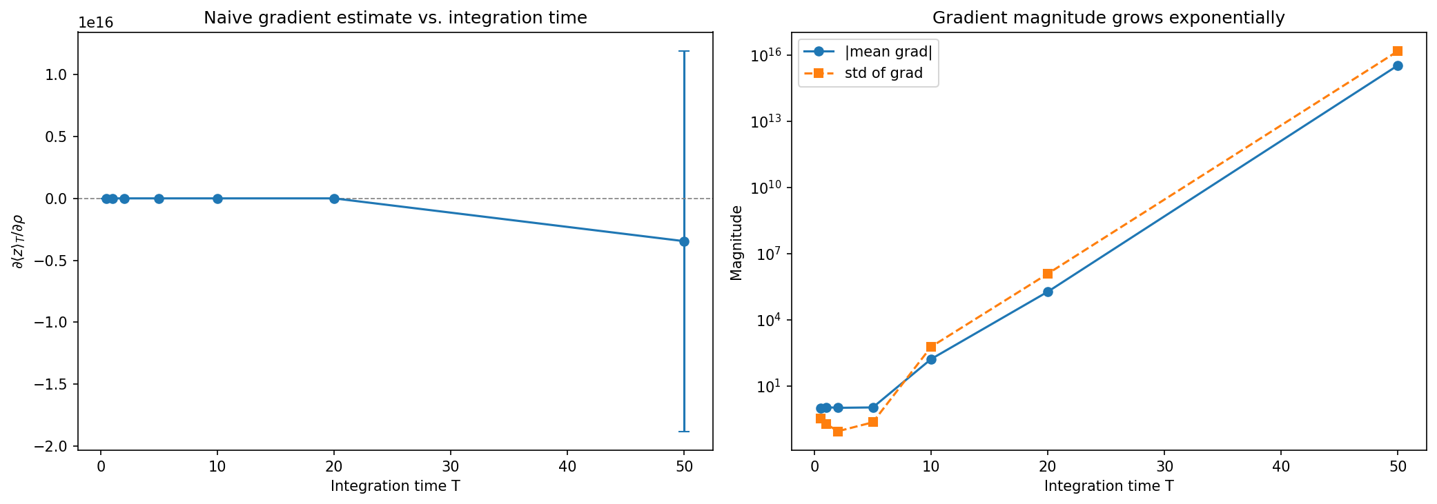
JAX makes it easy to differentiate through a simulation. However, this convenience does not help in chaotic systems. Naive autodiff can produce exponentially growing gradients that do not reliably estimate the sensitivity of long-time averages.

return jax.grad(objective)(rho_val)

The objective is the finite-time average of the Lorenz \(z\) coordinate, and the parameter is \(\rho\).

For any fixed finite \(T\), this derivative is well defined, and jax.grad(objective)(rho_val) is the correct mechanism for computing it, assuming all operations inside objective are differentiable.

The problem is that Lorenz 63 is chaotic. The derivative of a later state with respect to \(\rho\) depends on the tangent dynamics along the trajectory:

Because nearby trajectories separate rapidly, these tangent sensitivities can grow very quickly with time. Therefore, the gradient obtained by backpropagating through the entire trajectory can become extremely large, noisy, and highly dependent on the initial condition. This makes it a poor estimator of the derivative of the invariant-measure average

We can see the instability from the following results:

Output:

T=  0.5 | mean grad = +1.0141e+00, std = 3.5329e-01
T=  1.0 | mean grad = +1.1143e+00, std = 1.9646e-01
T=  2.0 | mean grad = +1.0449e+00, std = 9.0405e-02
T=  5.0 | mean grad = +1.0874e+00, std = 2.3056e-01
T= 10.0 | mean grad = -1.7000e+02, std = 6.1133e+02
T= 20.0 | mean grad = +1.9138e+05, std = 1.2544e+06
T= 50.0 | mean grad = -3.4562e+15, std = 1.5350e+16

In order to compute reliable sensitivity estimates for long-time averages, we need to instead use techniques such as least-squares shadowing, which are beyond the scope of this post.

6. Further Reading

Lyapunov Characteristic Exponents (Lyapunov exponents) measure the average exponential rate of divergence of nearby trajectories in a dynamical system.

• If the system has a strange attractor, any two trajectories \(\mathbf{x}(t) = \Phi^t(\mathbf{x}_0)\) and \(\mathbf{x}(t) + \delta \mathbf{x}(t) = \Phi^t(\mathbf{x}_0 + \delta \mathbf{x}_0)\) that start out very close will separate exponentially in time.
• This sensitivity to initial conditions is quantified by:

where \(\lambda\), called the leading Lyapunov exponent, represents the mean rate of separation.

Here are some resources that I found useful:

1. Largest Lyapunov Exponent using Autodiff in JAX/Python
2. Full Lyapunov Spectrum of Chaotic Lorenz System using JAX

References

1. JAX documentation
2. Alex McKinney, “On Learning JAX - A Framework for High Performance Machine Learning”
3. Aleksa Gordic, “Get Started With JAX”
4. Mathwords, “Dynamical System — Definition, Formula & Examples”
5. P. Cvitanovic, R. Artuso, R. Mainieri, G. Tanner, and G. Vattay, Chaos: Classical and Quantum, ChaosBook.org, Niels Bohr Institute, Copenhagen, 2020.
6. Y. Saiki and M. Yamada, “Time-averaged properties of unstable periodic orbits and chaotic orbits in ordinary differential equation systems”, Physical Review E 79, 015201(R), 2009.
7. M. Viana and K. Oliveira, Foundations of Ergodic Theory, Cambridge Studies in Advanced Mathematics, Cambridge University Press, 2016.
8. Wikipedia, “Attractor”
9. Wikipedia, “Dynamical system”