Recursive Types and Infinite Trees (Part 1 of 2)

Types in programming languages correspond to sets of semantic objects. Simple types, like int or string, have a clear meaning. However, recursive types, whose descriptions are self-referential with the \(\mu\) operator, can be challenging to grasp. This PLSE blog post aims to clarify the concept of recursive types by grounding the meaning of the \(\mu\) operator in terms of regular infinite trees.

Keywords: Types, Recursion, Infinite Trees, Automata

Background

This research adventure is inspired by an exercise problem in the Static Program Analysis textbook (SPA) by Anders Møller and Michael I. Schwartzbach. We first introduce the related context from the book.

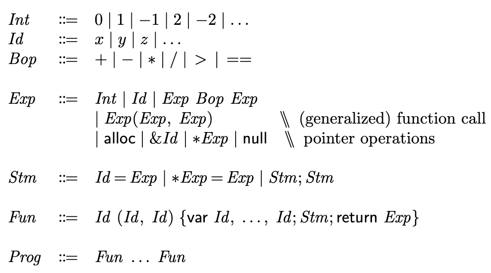
SPA works with a tiny imperative programming language, TIP. For this post, we only consider integers, pointers, functions with exactly two arguments, and assignments. More formally:

The goal of Chapter 3, Type Analysis, in the book is to infer types for all expressions. SPA first introduces a simple syntax of types with only three constructors:

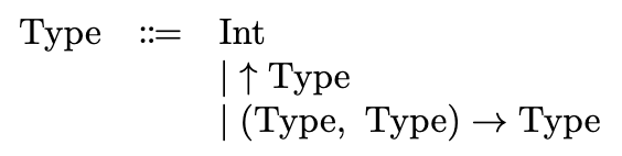
The \(\uparrow\) constructor is for pointers, e.g., \(\uparrow \mathrm{Int}\) denotes the type that is a pointer pointing to an \(\mathrm{Int}\) value.

Interpreting this as an inductive definition, a type is just a finite syntax tree, where each vertex of the tree is one of the three constructors with the corresponding number of children.

The need for infinite types

However, the finite types defined by induction are not enough to give types to recursive functions. Consider the following TIP program with function foo from Section 2.2 of the textbook, which computes the factorial in an unnecessarily complex way:

foo(p, x) {
  var q, f;
  if (*p == 0) {
    f = 1;
  } else {
    q = alloc 0;
    *q = (*p) - 1;
    f = (*p) * (x(q, x));
  }
  return f;
}

main() {
  var n;
  n = input;
  return foo(&n, foo);
}

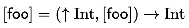
Although the function foo’s abstract syntax tree is finite, if we attempt to spell out its type, we would run into the issue that the second argument of foo can be the function itself. More precisely, the type of foo, \([\mathsf{foo}]\), must satisfy:

This equation is derived from the type-constraint rules defined in Section 3.2 of SPA and simplifying the constraints with substitution. Section 3.3 of SPA also lists all the constraints for this example program.

No finite type can satisfy this equation. If that were the case, then the size of the right-hand side of the equation would be strictly greater than that of the left-hand side, leading to a contradiction.

Section 3.1 of SPA describes an infinite solution to this equation:

But this answer is unsatisfactory: “…” is not part of the type syntax, and this infinite type is obviously out of the scope of the inductive definition (though it is in scope if we interpret the syntax definition coinductively, see Remark 1). It is also unclear how one would derive this solution, or whether it is a valid solution to the equation at all. (Hint: the unification algorithm for type checking is not the answer, but rather, its correctness assumes the existence of such a solution, see Remark 2.)

Infinite types as infinite trees

As finite types are finite trees, infinite types, such as the one with “…” above, can be understood as infinite trees. There are many equivalent definitions of infinite trees. We use the following:

Let \(D = {0, 1, \dots, n - 1}\), the set of first \(n\) natural numbers. Let \(D*\) be the set of all finite sequences where each element in the sequence is an element of \(D\). A subset \(S\) of \(D*\) is called prefix-closed iff for any sequence \(s \in S\) and any sequence \(s’\) that is a prefix of \(s\), we have \(s' \in S\).

Here is a concrete example of this definition:

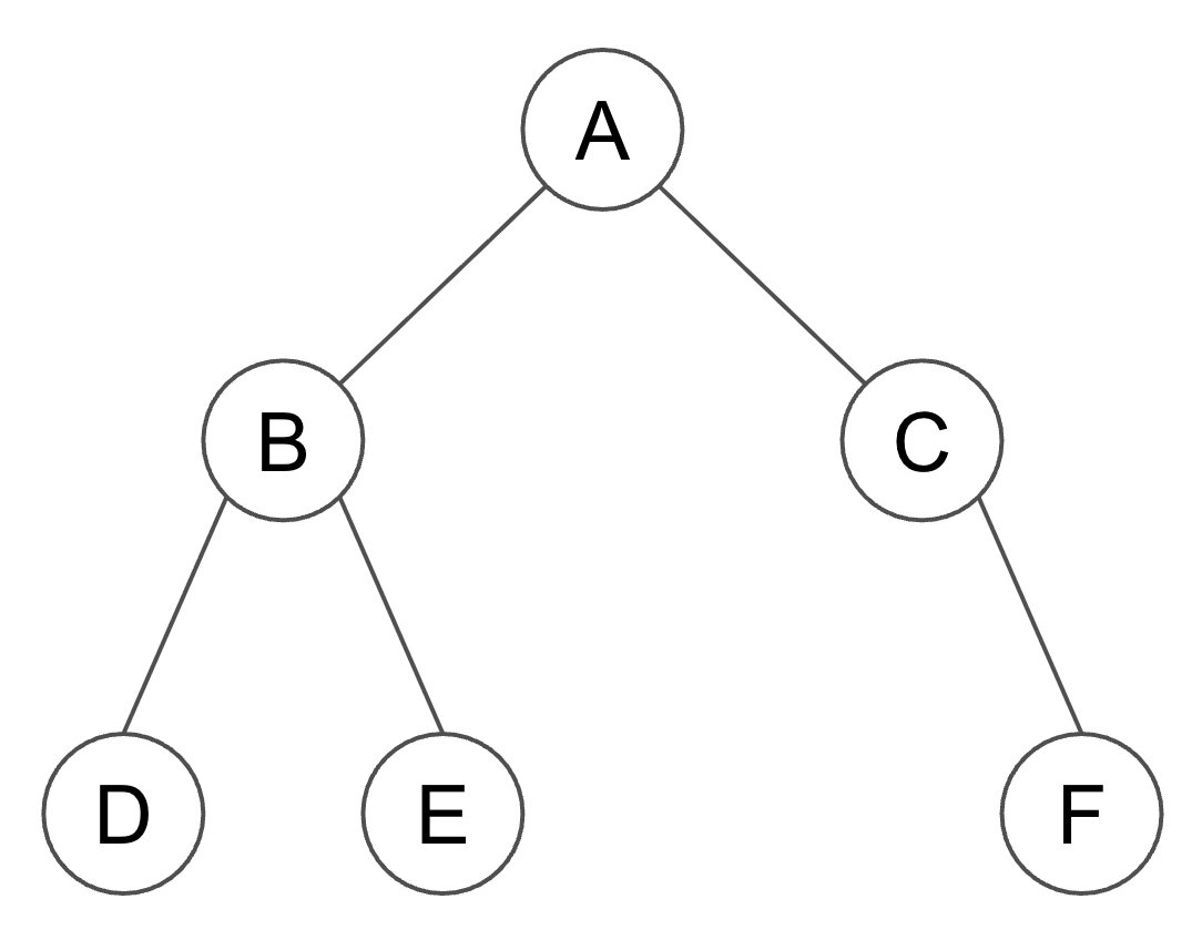
In this case, we have a binary tree, \(n = 2\), and \(D = \{0, 1\}\). The set \(S \subset D*\) that corresponds to the domain of this tree is \(\{\epsilon, 0, 1, 00, 01, 11\}\). The elements are the nodes \(A, B, C, D, E, F\). The set \(S\) is prefix-closed, which is equivalent to the condition that every node except the root must have a parent.

A tree is a function from a prefix-closed subset of \(D*\) to an arbitrary set of symbols, called an alphabet. A tree is finite if the number of elements in its domain as a function is finite, and infinite if its domain is infinite.

For our purpose, the alphabet is the set of type constructors. And we only need to set \(n\) to be the maximum arity (i.e., the maximum number of arguments) of all type constructors to distinguish the children of a tree node/arguments to a type constructor. For TIP, we set \(n = 3\) because the function constructor takes three arguments (two ordered inputs and one output).

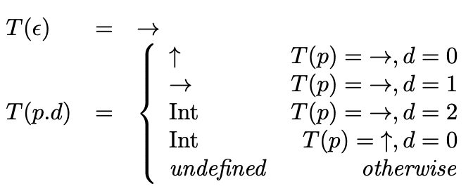
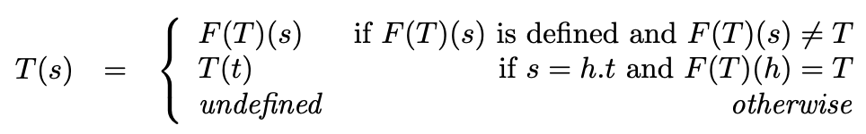
This definition allows us to precisely characterize infinite types as functions with infinite domains, using only finite-length syntax. Given the infinite type mentioned above, we can define it using the following recursive function \(T(x)\). We use the notation \(p.d\) to denote a sequence whose last element is \(d\) and the prefix sequence before \(d\) is \(p\). \(\epsilon\) denotes the empty sequence.

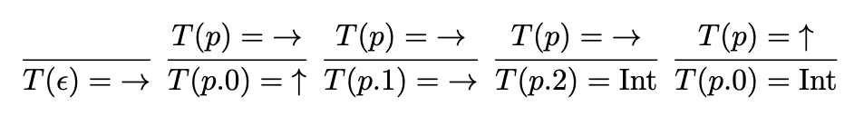
Equivalently, we can use our good ol inference rules for this kind of inductive definition:

Infinite trees as solutions to recursive type equations

With this precise definition, we can now formally reason about those types. As an example, we show that it is indeed a solution to the equation:

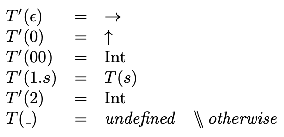
The left-hand side is just \(T\). The syntax tree of the right-hand side essentially describes a finite tree with some leaf nodes being \(T\). This derives the following definition for a function \(T'\), which refers to the definition of \(T\):

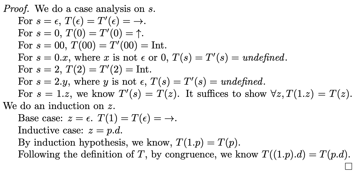
To show \(T\) is a solution to this equation, we show \(\forall s \in D*, T(s) = T' (s)\).

In fact, the way we derived \(T'\) can be generalized to construct an infinite tree solution to any equation of the form \(T = F(T)\), where \(T\) is a type variable and \(F(T)\) is a finite tree of type constructors and \(T\) treated as a constructor of arity \(0\) (so it can only show up at leaves). For the constructed solution to be well-formed, the finite tree \(F\) must follow the arity of the type constructors and must not just be \(T\) itself:

Conceptually, this construction is just repeatedly applying the original equation to substitute the type variables in its right-hand side. Or, “just spelling out the ‘…’.” But treating the infinite types as functions allows us to do so precisely without existential doubt.

Importantly, this construction always yields the unique solution to the equation, providing a foundation for the correctness of the unification algorithm (see Remark 2). As per the courtesy of the SPA textbook, the very important proof and some other critical properties are left as an exercise for the interested reader:

Exercise 1: Show that \(T\), as defined, is indeed a solution to the type equation \(T = F(T)\).

Exercise 2: Show that \(T\) is the unique solution to the type equation. That is, \(\forall T’, T’ = F(T’) \Rightarrow \forall s. T’(s) = T(s)\).

Exercise 3: Sketch how this construction can be generalized to a set of type variables \(T_1, T_2, \dots, T_m\) and a set of type equations

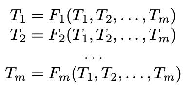
where each \(F_i\) is a finite tree of type constructors and type variables \(T_1, T_2, \dots, T_m\), and is not just a single type variable. This generalization allows one to handle mutually recursive types.

The \(\mu\) operator and regular trees

Defining infinite types as functions is helpful yet cumbersome. But now we know that any equation of the form \(T = F(T)\) (or a system of equations, as mentioned in Exercise 3) has a unique solution that can be derived syntactically.

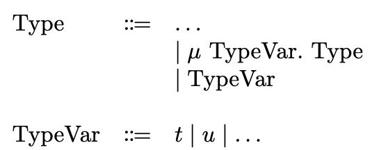
The key idea of the \(\mu\) operator is that we can use the equation as the syntax to name the infinite type that is the solution. This is more convenient than spelling out the function definition. We write \(\mu T. F(T)\) to denote this particular infinite tree that is the unique solution to the equation \(T = F(T)\). So we extend the syntax of types as in SPA:

Using this definition, the type of the function foo can be denoted as:

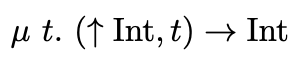
Which corresponds to the function \(T\) we just defined.

SPA’s definitions are a bit hand-wavy because they allow unbounded type variables and treat them as “any type”. A more stringent definition can be given by tracking the set of bounded variables.

An interesting observation of the \(\mu\) operator is that not all infinite trees can be named this way. This is because even with the \(\mu\) operator, all type expressions that follow this type syntax are essentially finite trees. So we can only name countably infinite many trees this way. But there are uncountably infinite many infinite trees.

For a more concrete example, consider the infinite binary tree where the right children form an infinite chain and the left children are full binary trees \(B_0\), \(B_1\), \(B_2\), …. This tree cannot be expressed using the \(\mu\) operator. One can show this by contradiction. Informally, suppose it is the solution to some equation \(T = F(T)\). By the definition of this tree, any path can only take a finite number of lefts, and for any finite number, there exists such a path that takes that many lefts. But since \(F\) is finite, there either exists a path that takes infinitely many lefts (if one can take a left turn in \(F\) and still reach a \(T\) leaf) or there exists an upper bound on the number of left turns a path can take (e.g., the height of $F$).

The truth is that the \(\mu\) operator can only be used to name infinite trees that have a finite number of subtrees up to isomorphism. (A subtree takes a node as the root and includes that node and all its descendants.) Such a tree is called a regular tree. And each regular tree is (an element of) the solution to some equational system that has the form \(T_i = F_i(T_1, …, T_m)\) as mentioned in Exercise 3.

Due to the English word “regular” being overloaded, it is essential to distinguish this concept of regular trees from other concepts that also have the word “regular” in them. For one thing, both ChatGPT and Gemini were very confused by the use of “regular” when I asked them to explain the concept of a regular tree. See Remark 3 for a laundry list of concepts with “regular” in their names for clarification.

Because TIP cannot define types in the program, and no type constraint rules use the \(\mu\) operator. It appears only when we explicitly name types that satisfy the constraint rules. In languages such as Haskell or OCaml, \(\mu\) may appear in the program to define recursive or mutually recursive types. Then the type analysis becomes more complex, requiring testing for equality between two infinite types. And in this case, we may use the automaton construction to help decide whether two infinite types are equivalent – a topic we will cover in a future blog post.

Remarks

Coinductive Definition

Abstractly, a definition is of the form \(X = F(X)\), where \(X\) is a set and \(F\) is a function from set to set.

In our case, \(\mathrm{Type}\) is a set, and \(F(X) = \{\mathrm{Int}\} \cup \{\uparrow\; t \mid t \in X\} \cup \{(x, y) \rightarrow z \mid x, y, z \in X\}\).

Informally, consider the power set lattice \(L\) of all possible terms, including all finite and infinite ones. \(F\) is a mapping from \(L\) to itself. It is not hard to see that this \(F\) is monotonic, i.e., it preserves the subset relations. By Tarski’s fixed point theorem, $F$ has a minimum fixpoint and a maximum fixpoint.

\(X = F(X)\), when interpreted as an inductive definition, names the minimum fixpoint, where every term is finite and grounded, i.e., can be derived from \(\emptyset\) in a finite number of iterations.

When interpreted as an coinductive definition, it names the maximum fixpoint. This would contain infinite terms such as \(\uparrow(\uparrow(\uparrow(\dots)))\) or \((\mathrm{Int}, \mathrm{Int}) \rightarrow ((\mathrm{Int}, \mathrm{Int}) \rightarrow \dots)\).

Unification

I suggest that the unification process is better understood as a simplification/normalization process rather than a solving process. It only goes so far as to reduce the set of input constraints to a form in which a solution is guaranteed to exist and never explicitly produces a concrete assignment to the type variables. More concretely, when unification terminates successfully, we only have a set of equalities represented by the state of the union-find data structure.

To see how the unification process described in SPA for TIP does guarantee a solution when it terminates successfully. We construct a system of equations of type variables in the normal form as described in Exercise 3 above.

A subtlety of the unification algorithm description in SPA is that it favors non-type variable expressions over type variables as the new representative when unioning two sets. This detail is crucial for correctness by guaranteeing each equivalence class can only be one of two cases: (1) Just type variables, in which case they must be free type variables that can take any type; (2) Contains at least one type expression that is not just a variable.

We first handle equivalence classes of case (1) by representing each with a single fresh symbol (not a fresh variable), \(A_i\). We then construct the system where each equation is of the form \(T_i = F_i(T_1, T_2, …, T_m)\) by making a fresh variable \(T_i\) for each equivalent class of case (2), where \(F_i\) is given by representative element of the equivalent class in the union find but with the original type variables substituted by \(A_i\)s or \(T_i\)s.

Then we can apply the construction of Exercise 3, which generalizes our construction of the unique solution to a single-variable equation to the unique solution to a multi-variable system.

All the “regular” things

Regular expressions (RE)

REs are the syntactic form of atom, union, concatenation, and Kleene star that describe a set of finite words of some alphabet.

Regular/Rational (finite) (word) languages

A finite word language is a set of finite words/strings of some alphabet A. A finite regular word language is a set of finite words that can be recognized by a deterministic finite automaton.

Kleene’s theorem shows the set of languages described by regular expressions is the same set of languages recognized by deterministic finite automata.

\(\omega\) regular expressions

Syntactic form with \(\omega\)-star, \(\omega\)-concat, and union.

Regular/Rational Infinite/\(\omega\) (word) languages, a.k.a, \(\omega\)-regular languages

An infinite word language is a set of infinite words of some alphabet A. An infinite word can be thought of as a function from \(\mathcal{N}\) to A. A regular infinite word language is a set of infinite words that can be recognized by a nondeterministic Buchi automaton.

An extension of Kleene’s theorem shows that this set of languages is equivalent to the set described by \(\omega\)-regular expressions.

Regular/Rational (finite) tree languages

A finite tree language is a set of finite trees of a ranked alphabet. A regular tree language is a set of finite trees that can be recognized by a deterministic bottom-up tree automaton or nondeterministic top-down tree automaton.

Another extension of Kleene’s theorem shows that this set of languages is equivalent to the set described by regular tree grammar, or an alternative equivalent definition with tree concatenation and tree Kleene star.

Regular/Rational Infinite/\(\omega\) tree languages

An infinite tree language is a set of infinite trees of a ranked alphabet. A regular infinite tree language is a set of infinite trees that can be recognized by a nondeterministic (top-down) Buchi tree automaton.

Yet another extension of Kleene’s theorem shows that this set of languages is equivalent to the set of languages that can be described by a tree expression with \(\omega\)-star and \(\omega\)-concatenation.

Summary

Every combination of {finite, infinite} \(\times\) {tree or word} has its own Kleene’s theorem that ties the set of languages described by some grammar of some variations of atom, union, concatenation, and Kleene star to languages recognizable by some class of automaton.

The automatons have more categories. There are common vs. (Buchi, Muller, …), word vs. tree, and deterministic vs. nondeterministic. For finite tree automata, in particular, there is top-down vs. bottom-up.

It is also the case that the infinite languages usually refer to “purely” infinite ones that do not contain finite words/trees. For trees, that means all branches must be infinite. However, we do deal with “inpure” infinite trees here that are be finite on some branches. Those can be made pure by padding all finite branches with an infinite chain of some fresh character that is not in the original alphabet.

Mention that, all these uses of regular are applied to languages, which are sets of words or trees. So regular word/tree languages are sets of sets of words or trees. The regular tree we mentioned above is a specific set of trees. Rabin’s basis theorem gives a connection between the two. We will explain more next time with a more concrete definition of tree automatons.

Acknowledgements

I would like to give my special thanks to the following friends and mentors for helping me understand the materials and write the blog post: Dietrich Geisler, Michael Roberts, Andrew Myers, Josh Acay, \(\mathcal{N}\)(at) Hurtig, and Zachary Tatlock.

References

Anders Møller and Michael I. Schwartzbach (2024). Static Program Analysis (SPA).

Andrew Myers (2025). Cornell CS 6110 Lecture Notes.

Comon et;al (1999). Tree Automata Techniques and Applications.

C.-H. L. Ong (2013). Automata, Logic and Games.

Dominique Perrin and Jean-Éric Pin (2004). Infinite Words Automata, Semigroups, Logic and Games.