Managing Research Data with Databases and Interactive Visualization

Every project needs to store and visualize data. Most of us have generated a static plot with matplotlib from data in a CSV file. However, when the data format becomes slightly more complicated and the data size increases, both correctness and performance issues arise. This blog post will try to convince you that databases and interactive visualization provide a better pipeline. It is less error-prone, easier and faster to process your data, and has a shorter feedback loop, all without necessarily adding to your workload.

Is CSV that bad?

Yes, it is. Remember your hands shaking as you write in a language where you don’t even know a variable’s type? That is what CSV does to your data. Actually, you’d better not shake your hands when editing a CSV file, because just an extra space after a comma would turn the next integer into a string with a leading space. Eww! And that is just one of the many problems stemming from the untyped nature of the CSV format.

Using CSV is error-prone

A CSV file has no guarantees or format specification. Each line can have arbitrarily many columns, not necessarily the same as in previous lines. It is also not guaranteed that data in the same column is the same type. And worst of all, there is no way to know what the exact format is unless you read the code that generated this CSV file, which is usually a bunch of print calls scattered across the system! I understand that it is the easiest way to collect data from a system, and I do not oppose using CSV as a first step, but you may run into surprises if you use that unchecked CSV file.

Processing or filtering CSV is time-inefficient

Most CSV libraries read the entire table. Without index information, the library must look through all the data at least once, even if the library later builds an index. This is fine for small datasets, but it is slow when you scale up your experiments. Gigabytes of data are common in system logs.

Storing in CSV is space-inefficient

Since data is stored as characters in a CSV file, numbers usually take many times more disk space than they would in a binary format. This makes it even worse under the scenario that most processing requires reading the entire file.

Databases to the rescue

Despite all the benefits, people are still reluctant to use a database because it just sounds more heavyweight, and they believe it requires extra effort. I will try to convince you that the effort is tiny, and it saves you more time later on.

Building a database is easy

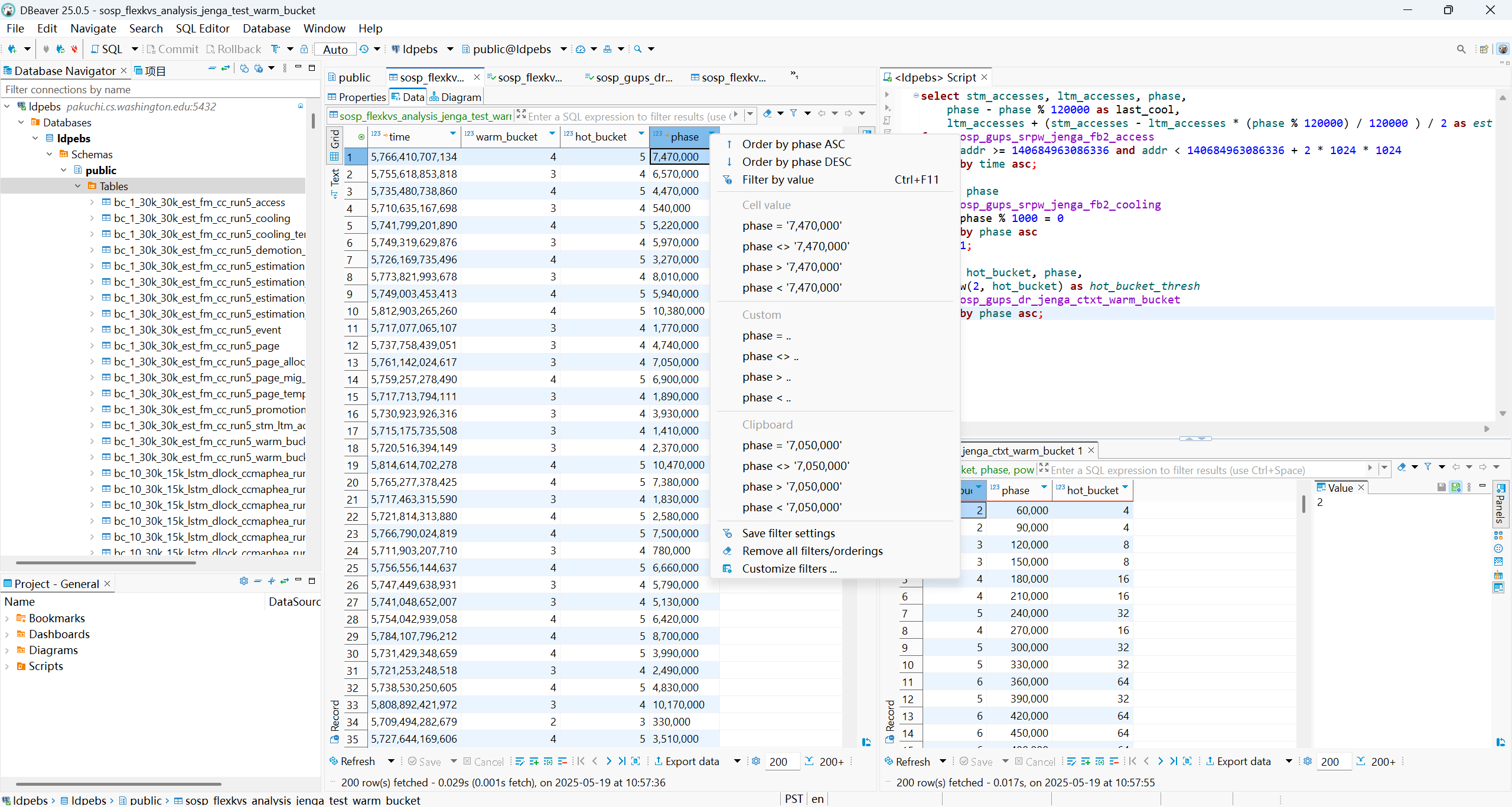
Now it is 2025, and you no longer need to build a database with command lines. There are very nice database management tools with a GUI, like DBeaver, that allow you to build a table and import from a CSV file in a few clicks. They also allow you to navigate through the data much like using a spreadsheet editor. You can try your queries in an integrated window, see the results on the same page, and navigate through them like a spreadsheet. Super convenient!

However, if you are more old-school about databases, you can use SQL scripts. I actually feel that it is faster than the GUI when you become a power user, because you can automate it with other scripts, and most important of all, LLMs write them well. The script below creates a table alloc and populates it with alloc.csv.

CREATE TABLE alloc (
    time int8 NOT NULL,
    addr int8 NOT NULL,
    hugepage int4 NOT NULL,
    phase int8 NOT NULL
);
\COPY alloc (time, addr, hugepage, phase) FROM './alloc.csv' WITH (FORMAT CSV, DELIMITER ',', NULL 'NULL');

Reading from a database is easy

Reading from a database is as easy as reading from a CSV file. I am using PostgreSQL as an example here, but if you want to preserve the single-file convenience of the CSV format, you can use SQLite instead.

db_connection = psycopg2.connect(
    dbname="dbname",
    user="user",
    password="password",
    host="localhost"
)
df_alloc = pd.read_sql("SELECT * FROM alloc", db_connection)

Database schema is a natural specification

Remember all the crazy CSV formats? You can say no to them in a database. By specifying the column types and nullness allowance when you build the table, you are already rejecting any broken rows from the raw data. Importing will fail if any of the rows violate the constraints, and you will know exactly which rows are problematic. You don’t have to wait until visualization to get a surprise. Totally sane!

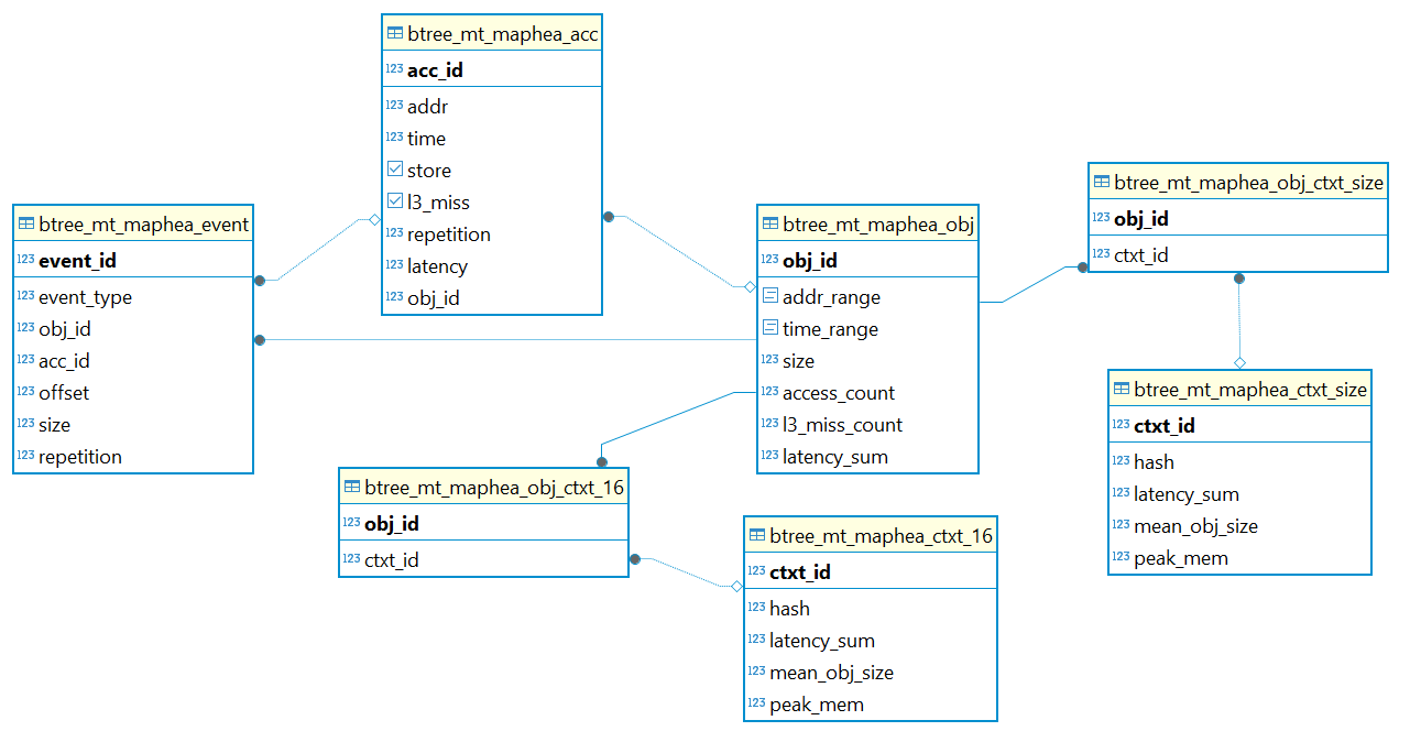
More importantly, the database schema now serves as a specification of your data format, with a nice-looking visualization for free from DBeaver. This is especially helpful as a contract if you are working with a collaborator or intend to distribute your data to a downstream user.

Databases also support more complicated constraints, such as data range restrictions and reference restrictions (foreign keys). You don’t have to make any extra effort if you don’t want it, but it’s always there when you need more sanity.

Data processing with a database is time-efficient

SQL is a powerful and highly optimized programming language. Many operations benefit from existing indices. For example, if you frequently query or process data within a certain time range, maintaining a B-Tree index on that column allows the database to read only slightly more than the range you need, rather than the entire table.

Though it may sound hard to write SQL, there is one trick that makes it much easier: using WITH ... AS ... clauses. They allow you to make a temporary query and assign it to a name, then use that temporary table to make further queries without storing those intermediate tables to disk. This trick makes my SQL programs more sequential (rather than deeply nested) and easier to understand. For example, if we want to subtract away the value of the smallest phase from the entire phase column, we can either do a nested query or a WITH ... AS ... query. The WITH ... AS ... query is longer, but logically it’s more like a sequential program and easier to read.

-- Traditional, nested, declarative SQL query
SELECT
  time, addr, hugepage,
  phase - (SELECT MIN(phase) FROM alloc) AS phase_normalized
FROM alloc;

-- SQL query using `WITH ... AS ...`
WITH min_phase AS (
  SELECT MIN(phase) AS value
  FROM alloc
)
SELECT
  a.time, a.addr, a.hugepage,
  a.phase - m.value AS phase_normalized
FROM alloc AS a, min_phase AS m;

Since we are all asking for data processing scripts from LLMs anyway, you should probably trust SQL scripts a bit more than CSV processing scripts they generate. Why? If something is obviously wrong—say, type mismatches—the database will tell you even before it starts executing. Also, you can be confident that your data is not modified as long as there are no INSERT or DROP keywords in the script.

A tip for using an LLM for SQL script generation is giving it context by copy-pasting the schema to it, essentially the CREATE TABLE queries. That way, it knows the exact names and types of data that it will be manipulating. It doesn’t matter even if you lost the initial CREATE TABLE queries, because DBeaver can help you generate that from an existing table.

If you really don’t like SQL, you can still fall back to reading the table into Python, processing it as you would with CSV, and writing it back into the database. The difference is that you get a guarantee that what you write back is still sane, without any surprise NaNs or NULLs.

Data storing with a database is space-efficient

Different from CSV’s character storage, databases use binary formats by default. The difference becomes obvious when each of your CSV files has gigabytes of data—not only because it saves disk space, but also because it saves disk I/O time. If you have even more data than that, mainstream databases also support enabling data compression with just one configuration change.

How to remove columns

If you have some trash columns in your raw data that you want to get rid of, you can first create a temp table, then copy certain rows from that temp table, and finally drop the temp table. You can do it with SQL scripts or with a GUI.

\COPY alloc_temp(trash0, time, addr, hugepage, phase) FROM './alloc_with_trash.csv' WITH (FORMAT csv, DELIMITER ',', NULL 'NULL');
CREATE TABLE alloc_temp (
    trash0 int4 NOT NULL,
    time int8 NOT NULL,
    addr int8 NOT NULL,
    hugepage int4 NOT NULL,
    phase int8 NOT NULL
);
INSERT INTO alloc (time, addr, hugepage, phase) SELECT * FROM alloc_temp;
DROP TABLE alloc_temp;

More accurate data understanding with interactive visualization

“Interactive visualization” means plots that allow you to zoom in and enable or disable certain elements without modifying your plotting script.

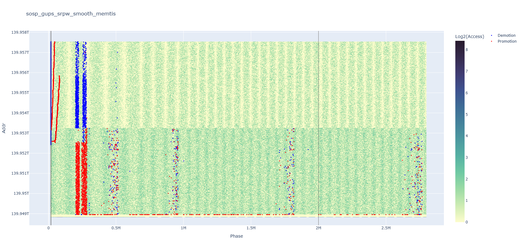
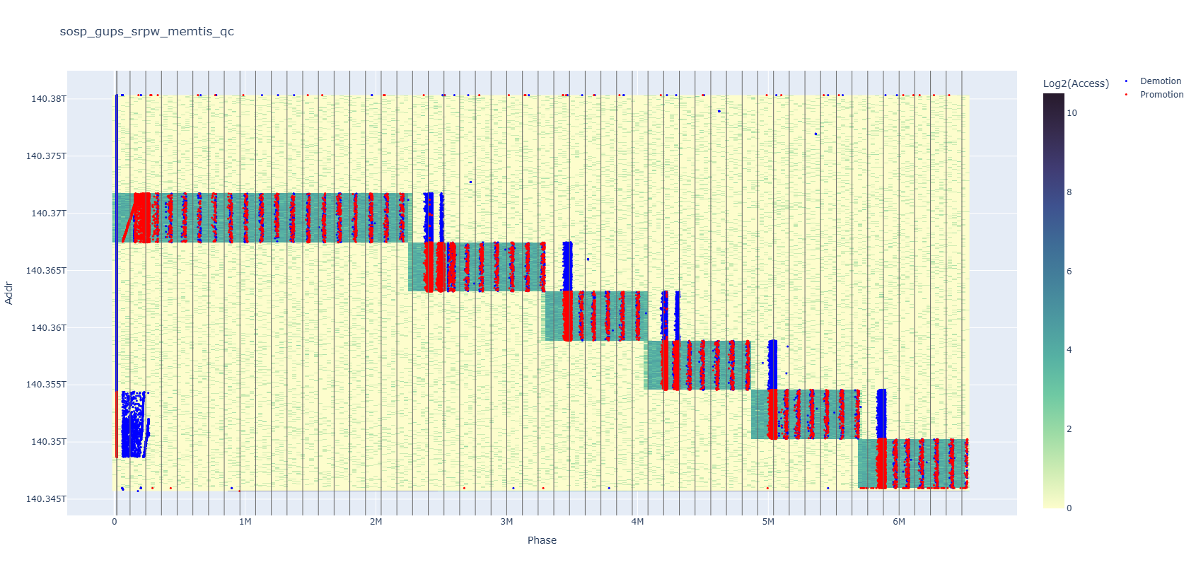
Your data can lie to you if you don’t look carefully enough. The above plot is a memory heatmap with the x-axis representing time and the y-axis representing addresses, overlaid with red and blue dots each standing for a kind of memory event. At the left end of the plot, the red dots seem to occur in increasing address order, right?

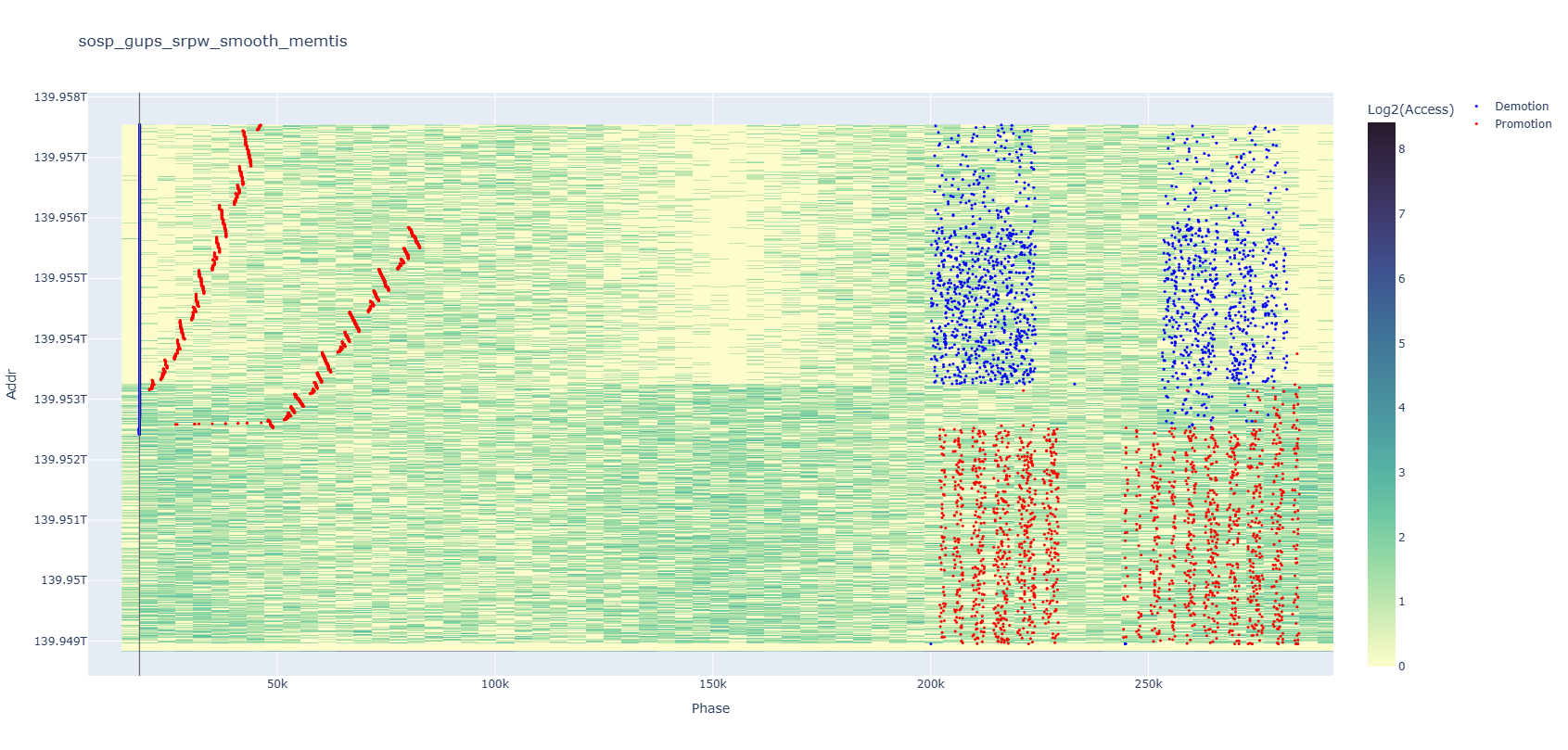
If you zoom in, you will quickly realize that’s not true. It is in an increasing address order as a big trend, but every small segment is actually in reverse order, similar to how Okazaki fragments perform DNA replication. You can also notice some internal patterns appearing among events on the right after zooming in.

With an interactive window, it is instinctive to zoom in on interesting parts of a plot. But if that requires you to modify and rerun your SQL or CSV script and plotting script, won’t there be a moment when you want to give up, since the plot already looks fine?

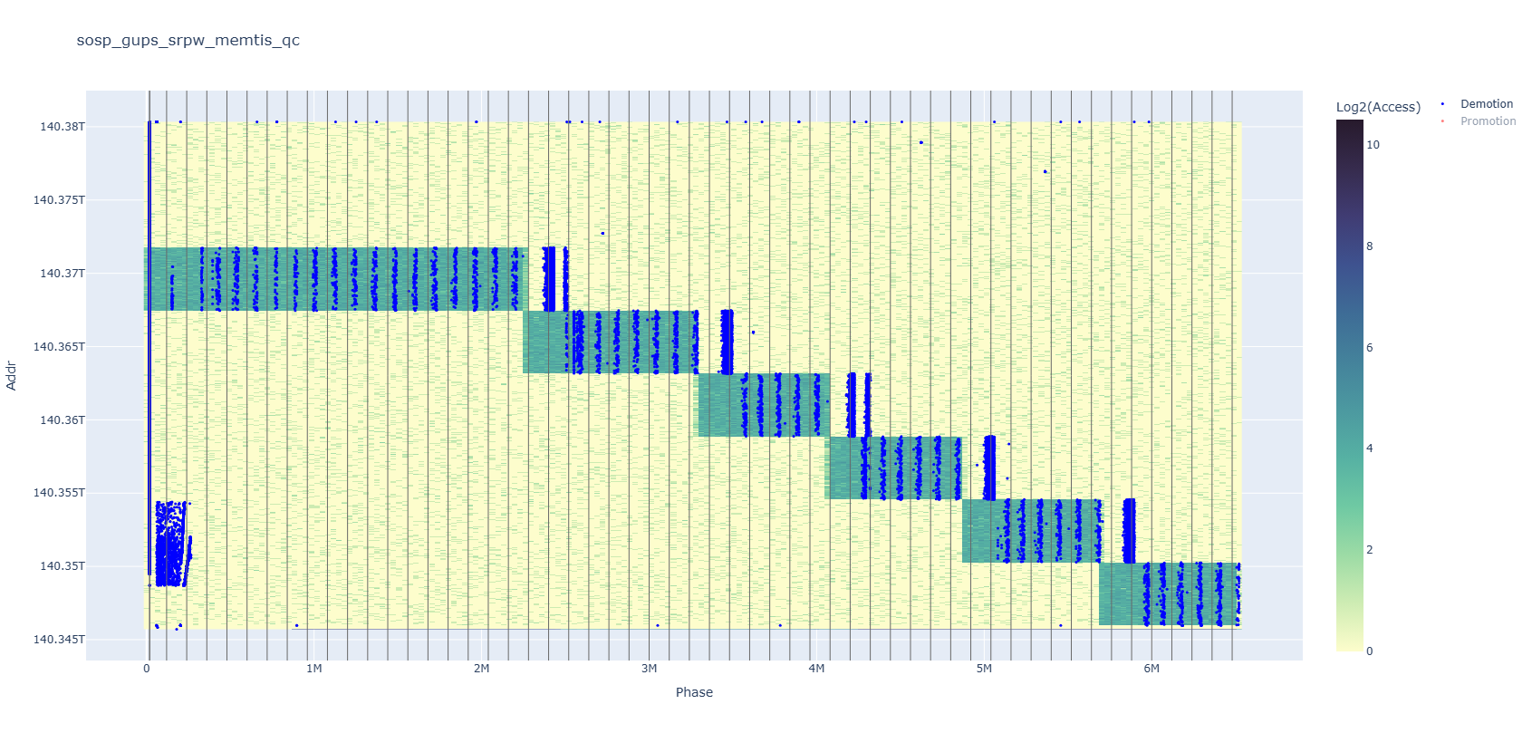
Here is another example. At first glance, it seems that red dot events dominate the heatmap, but if you turn off the red series, you’ll find that there are just as many blue dots—many of which were hidden behind. Compared to clicking a mouse, having to modify and rerun the plotting script to remove half of the data—which is especially slow if you are using CSV, which does not have an index on the tag column—undoubtedly harms people’s interest in trying it.

Visualization is super important, and being able to fully understand your plots is just as important. No exaggeration, but all my research contributions to one project literally came from observing imperfections in previous systems’ behavior, which was revealed through these plots.

Switching to an interactive visualization is an investment in data analysis, which will repay itself many times over. More important than saving overall time, it prevents my chain of thought about system design from being interrupted by technical details. I greatly appreciate how interactive visualization helps me focus.

Choosing a dynamic visualization library over a static one has literally no cost. Their APIs are similar, and better news is that LLMs are very good at writing them. I am using plotly here, and matplotlib also has an interactive functionality. I am not going to talk about how to use them in detail, because the most important thing here is to make the right choice when you start.

Conclusion

In short, moving beyond CSV files to a database-backed workflow with interactive visualization transforms your research data pipeline from error-prone and slow into a self-validating, self-documenting system. By defining a clear schema, you eliminate type and format errors at import time; by leveraging indexes and optimized queries, you speed up filtering and aggregation; and by switching to interactive plots, you speed up your exploration of data without repeated script edits. Best of all, getting started takes only a few clicks or a handful of SQL commands, and with LLMs ready to draft both your database scripts and your plotting code, it costs almost no extra effort. Please give this approach a try, and you won’t regret it!

Acknowledgements

Thanks to Rohan Kadekodi for the project we did together that inspired all my thoughts about research data management. Also thanks to Haobin Ni and Michael Ernst for editing this blog post.