Taxonomy of Small Floating-Point Formats
Post Metadata
As part of my responsibilities as an industrial PhD student with PLSE and Intel, I develop and maintain, alongside my colleague and PLSE alumni Bill Zorn, a reference implementation of floating-point arithmetic. Hardware designers use this reference model to formally specify the behavior of floating point in hardware designs and verify the correctness of their implementations of these designs. Our library must not only have reasonable performance while simulating these designs and be consumable by formal verification tools for equivalence checking or property verification; but it must also correctly answer the often difficult question about floating point: “but what do it do?” With the prevalence of machine learning and its demand for ever smaller number formats for increased performance, we explored the interesting and often ridiculous world of small floating-point formats.
This post is split into three parts:
- The IEEE 754 standard and floating-point terminology.
- Recent proposals and standards floating-point formats beyond IEEE 754.
- Small floating-point formats and their properties.
IEEE 754 standard
As brief background, I will review the IEEE 754 standard and cover basic floating-point terminology. Introduced in 1985 (with revisions in 2008 and 2019), it was the first widely-used standard for floating-point arithmetic. So universal was its adoption, it described the only standard floating-point formats available across different hardware architectures until the recent introduction of the Open Compute Project (OCP) Microscaling Formats (MX) Specification and the upcoming standard from the IEEE P3109 working group, both addressing limitations of IEEE 754 for small number formats.
Floating-Point as Numbers
I will present two equivalent views of a floating-point value, say \(x\). Keep in mind that we are in base 2! In the “unnormalized” view, \(x\) consists of a sign \(s\), an exponent \(exp\), and integer significand \(c\)
\[x = {(-1)}^s \times c \times 2^{exp}.\]In the “normalized” view, \(x\) instead consists of an exponent \(e\) and fractional significand \(m\), also called the mantissa.
\[x = {(-1)}^s \times 1.m \times 2^{e}.\]We say that \(x\) is in the binade of exponent \(e\), i.e., the interval \([2^e, 2^{e+1})\). In rare cases, specifically when \(e\) is the smallest possible value \(e_{\text{min}}\) according to the number format, \(x\) is represented by
\[x = {(-1)}^s \times 0.m \times 2^{e_{\text{min}}}.\]When \(e = e_{\text{min}}\) and \(m \neq 0\), we say that \(x\) is a subnormal number. When \(e > e_{\text{min}}\), we say that \(x\) is a normal number.
The term precision refers to the number of digits required to encode \(c\) and \(m\). We say that \(x\) has precision \(p\) when \(c\) requires \(p\) digits to represent it (equivalently, \(m\) requires \(p-1\) digits to represent it). When converting from the normalized view to the unnormalized view, we shift the digits of \(1.m\) (or \(0.m\)) left by \(p - 1\) to form \(c\), which now has no fractional digits; and then set \(exp = e - p + 1\). The opposite is mostly straightforward, keeping in mind the special case of subnormal numbers.
\[{(-1)}^0 \times 1.01 \times 2^0 \quad\Leftrightarrow\quad {(-1)}^0 \times 101. \times 2^{-2}.\]Above is a possible representation of the number 1.25 in a normalized (left) and unnormalized (right) view with 3 digits of precision. Keep in mind, the mantissa is in base 2! For this example, we shift by \(p - 1 = 2\) when converting between the two representations.
Floating-Point as Bitstrings
In addition to representing numbers, floating-point values must also be represented in memory as a sequence of bits.
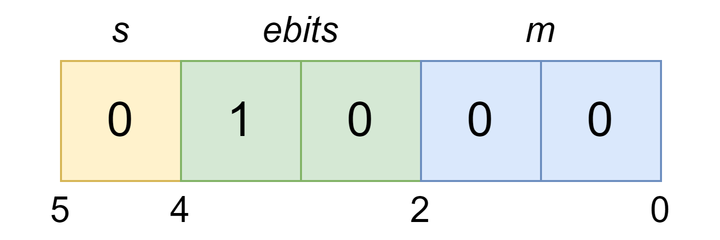
The figure above shows a small floating-point format with only 2 bits for the exponent and 2 bits for the (fractional) significand. We parameterize IEEE 754 formats by the size of the exponent field, \(es\), and the total size of the format, \(nbits\). We interpret the fields \(s\) and \(m\) in the manner described before. Interpreting the exponent field \(ebits\) is less straightforward. When \(ebits\) is 0, \(x\) is a subnormal value (or zero!). If \(ebits = 2^{es} - 1\) (all ones), then \(x\) is a special value (e.g., infinity or NaN) with \(m = 0\) encoding infinity and \(m \neq 0\) encoding NaN. Otherwise, \(x\) is a normal value and \(e = e_{\text{min}} + ebits - 1\). Roughly, \(x\) is \(ebits-1\) binades away from the binade of exponent \(e_{\text{min}}\), excluding the special case of subnormal numbers (see Appendix, “Exponent Bias” for further commentary).
We list the common IEEE 754 formats below with their format parameters as well as derived parameters like the precision of normal numbers \(p\), minimum (normalized) exponent \(e_{\text{min}}\), and maximum (normalized) exponent \(e_{\text{max}}\).
| Format | Aliases | es |
nbits |
p |
e_min |
e_max |
|---|---|---|---|---|---|---|
float<15, 128> |
quad, binary128 | 15 | 128 | 113 | -16382 | 16383 |
float<11, 64> |
double, binary64 | 11 | 64 | 53 | -1022 | 1023 |
float<8, 32> |
single, binary32 | 8 | 32 | 24 | -126 | 127 |
float<5, 16> |
half, binary16 | 5 | 16 | 11 | -14 | 15 |
We compute the derived quantities as follows:
\[p = nbits - es,\quad e_{\text{max}} = 2^{es-1} - 1,\quad e_{\text{min}} = 1 - e_{\text{max}}.\]The IEEE 754 standard adds additional structure to NaN values. The standard identifies the top most bit of \(m\) to be the quiet bit, and the remaining bits to be the payload which can carry diagnostic information (see C/C++ nan/nanf/nanl). When the quiet bit is set, the NaN value is a quiet NaN (qNaN). Otherwise, the NaN value is a signaling NaN (sNaN); the standard specifies that sNaN values may optionally raise an exception when used in arithmetic operations. A subtle constraint is that any sNaN must have a non-zero payload. Otherwise, \(m = 0\) and the value would encode infinity.
For illustrative purposes,
a table of values (ignoring sign)
of float<2, 5> are shown below.
The mantissa is represented in binary
and in decimal (in parentheses);
the “X” in the bits column represents the sign bit.
For NaN values,
the type of NaN and payload are shown.
| bits | e | 1.m / 0.m | exp | c | x |
|---|---|---|---|---|---|
| 0bX0000 | 0 | 0.00 (0.0) | -2 | 0 | 0 |
| 0bX0001 | 0 | 0.01 (0.25) | -2 | 1 | 0.25 |
| 0bX0010 | 0 | 0.10 (0.50) | -2 | 2 | 0.5 |
| 0bX0011 | 0 | 0.11 (0.75) | -2 | 3 | 0.75 |
| 0bX0100 | 0 | 1.00 (1.0) | -2 | 4 | 1 |
| 0bX0101 | 0 | 1.01 (1.25) | -2 | 5 | 1.25 |
| 0bX0110 | 0 | 1.10 (1.5) | -2 | 6 | 1.5 |
| 0bX0111 | 0 | 1.11 (1.75) | -2 | 7 | 1.75 |
| 0bX1000 | 1 | 1.00 (1.00) | -1 | 4 | 2 |
| 0bX1001 | 1 | 1.01 (1.25) | -1 | 5 | 2.5 |
| 0bX1010 | 1 | 1.10 (1.50) | -1 | 6 | 3 |
| 0bX1011 | 1 | 1.11 (1.75) | -1 | 7 | 3.5 |
| 0bX1100 | - | - | - | - | \(\infty\) |
| 0bX1101 | - | - | - | - | sNaN(1) |
| 0bX1110 | - | - | - | - | qNaN(0) |
| 0bX1111 | - | - | - | - | qNaN(1) |
Alternatively, we can display each value (ignoring sign) on a two-dimensional grid, which I will call a binade table, with each mantissa value arranged horizontally and each binade arranged vertically.
ebits \ m |
0x0 | 0x1 | 0x2 | 0x3 |
|---|---|---|---|---|
| 0x3 | \(\infty\) | sNaN(1) | qNaN(0) | qNaN(1) |
| 0x2 | 2 | 2.5 | 3 | 3.5 |
| 0x1 | 1 | 1.25 | 1.5 | 1.75 |
| 0x0 | 0 | 0.25 | 0.5 | 0.75 |
This view of floating-point values is particularly useful when exploring small floating-point formats. Note that numerical values increase in magnitude from bottom to top and left to right.
Beyond IEEE 754
Before jumping into our survey of small floating-point formats, we must examine recent history of floating-point formats beyond the IEEE 754 standard. Specifically, how have recent proposals for new floating-point formats broken from the IEEE 754 standard? And how might these new formats inform what could come next?
Since the introduction of the IEEE 754 standard, hardware designers introduced additional floating-point formats beyond those explicitly in the standard including Pixar’s PXR24 format and AMD’s fp24 format introduced for graphics applications in the 1990s and 2000s; and later Nvidia’s TensorFloat-32 format and Google’s bfloat16 format in the late 2010s for machine learning. These formats are smaller than the IEEE 754 single-precision format and thus offer better performance at the cost of precision. This push for smaller formats led to the addition of the half-precision format in the 2008 revision of the IEEE 754 standard. Despite this, the IEEE 754 standard still sufficiently describes these formats; the table below shows their parameters:
| Format | Aliases | es |
nbits |
p |
e_min |
e_max |
|---|---|---|---|---|---|---|
float<8, 24> |
PXR24 | 8 | 24 | 16 | -126 | 127 |
float<7, 24> |
fp24 | 7 | 24 | 17 | -62 | 63 |
float<8, 19> |
TensorFloat-32 | 8 | 19 | 11 | -126 | 127 |
float<8, 16> |
bfloat16 | 8 | 16 | 8 | -126 | 127 |
Recently, proposals for new floating-point formats beyond the IEEE 754 standard have emerged. Graphcore published their 8-bit (FP8) floating-point standard in June 2022. Nvidia, ARM, and Intel published their proposal in September 2022. These efforts culminated in the approval for the IEEE P3109 working group to develop an official 8-bit float standard in February 2023. Later, the Open Compute Project (OCP) Microscaling Formats (MX) specification in September 2023 which introduces 8-bit, 6-bit (FP6), and 4-bit (FP4) formats. Without consensus on a new standard by the IEEE, the OCP MX specification is now the current industry standard for floating-point formats 8 bits and smaller. To understand these new formats, we must first understand the limitations of the IEEE 754 standard.
Why so many NaNs?
Recall that IEEE 754 compliant NaN values use the mantissa to store diagnostic information. In practice, this information is rarely used, so having different NaN values is unnecessary. This redundancy is barely noticeable for larger formats, but becomes costly for smaller formats. Below is a table showing the number of NaN values for different IEEE 754 formats and the percentage of encodings.
| Format | # NaNs | % NaNs |
|---|---|---|
float<11, 64> |
9 007 199 254 740 990 | 0.0488 |
float<8, 32> |
16 777 214 | 0.391 |
float<5, 16> |
2 046 | 3.12 |
float<4, 8> |
14 | 5.47 |
float<2, 5> |
6 | 18.75 |
There are a number of proposed solutions for this issue.
NaN has mantissa of all ones.
When the exponent field is all ones, rather than allowing any non-zero mantissa to encode NaN, we only allow the all ones mantissa to encode NaN. This reduces the number of NaN encodings to 2, one for each sign: +NaN and -NaN. This solution is used in the MX specification for encoding the FP8 format with 4 bits of exponent.
For the remaining encodings,
we may encode infinity to be the “previous” value
(its mantissa is all ones minus one)
while all other encodings now represent normal values
in the binade of \(e_{\text{max}} + 1\).
These values grant the format an additional
binade which is important for very small formats
with only a few binades of values.
While these values are treated no differently
than other normal values, I will call them
supernormal values to distinguish them.
Below is part of the encoding table
for float<2, 5> modified with this solution;
“NaN” represents the NaN value with all ones mantissa;
supernormals have a normalized exponent of \(e = 2\).
| bits | e | 1.m / 0.m | exp | c | x |
|---|---|---|---|---|---|
| … | … | … | … | … | … |
| 0bX1011 | 1 | 1.11 (1.75) | -1 | 7 | 3.5 |
| 0bX1100 | 2 | 1.00 (1.00) | 0 | 4 | 4 |
| 0bX1101 | 2 | 1.01 (1.25) | 0 | 5 | 5 |
| 0bX1110 | - | - | - | - | \(\infty\) |
| 0bX1111 | - | - | - | - | NaN |
NaN replaces negative zero.
Looking at a table of floating-point values,
we notice the peculiarity of having two zero values:
one positive and one negative.
The reasons for having two zeros are somewhat out of scope,
but it causes issues in programming languages
that distinguish numerical and representation equality
(as does NaN).
For most applications though,
two zeros is unnecessary, so we can
replace negative zero with NaN.
This solution is used for Graphcore’s FP8 formats.
For the remaining encodings,
infinity may be the “largest” value
(its mantissa is all ones)
while all other encodings now represent normal values.
Below is part of the encoding table
for float<2, 5> modified with this solution;
“NaN” represents the NaN value replacing -0.
| bits | e | 1.m / 0.m | exp | c | x |
|---|---|---|---|---|---|
| 0bX0000 | 0 | 0.00 (0.0) | -2 | 0 | 0 / NaN |
| … | … | … | … | … | … |
| 0bX1011 | 1 | 1.11 (1.75) | -1 | 7 | 3.5 |
| 0bX1100 | 2 | 1.00 (1.00) | 0 | 4 | 4 |
| 0bX1101 | 2 | 1.01 (1.25) | 0 | 5 | 5 |
| 0bX1110 | 2 | 1.01 (1.50) | 0 | 6 | 6 |
| 0bX1111 | - | - | - | - | \(\infty\) |
No NaN values.
Perhaps a more radical solution is to
remove NaN values entirely.
In practice,
NaN results are unusable,
representing a complete error in computation.
Moreover,
NaNs propagate, causing all
future computations to be NaN.
For certain applications,
it may be more desirable to return some
numerical value rather than returning NaN.
This solution is used in the MX specification
for encoding 6-bit and 4-bit formats.
The encoding table for float<2, 5> modified
with this solution is similar to the previous one;
NaN is simply dropped.
Do we even need infinities?
In the IEEE 754 standard, infinities represent exact infinities, i.e. 1/0, or a number that is too large in magnitude (this condition is called overflow.). While useful in some applications, they may easily produce NaNs when used in later computations. For example,
\[\infty + (-\infty) = \text{NaN}, \quad \infty - \infty = \text{NaN}, \quad \infty \times 0 = \text{NaN}, \quad \infty / \infty = \text{NaN}.\]Rather than producing infinities,
we may instead produce the largest representable value
with the correct sign,
a trick known as saturation.
While the result likely has arbitrary rounding error,
it is still a numerical value,
and is unlikely to produce NaNs in later computations.
When removing infinities from a format,
the value is replaced with the next largest value
by the format.
For example,
in the previous encoding table for float<2, 5> with no NaN values,
the infinity would be replaced by the value \(x = 7\).
The MX specification requires a saturation mode
for both 8-bit formats, while requiring saturation
for 6-bit and 4-bit formats.
Why have a fixed exponent range?
The IEEE 754 standard imposes a fixed bound on the possible exponent values that are computed directly from format parameters. While reasonable for larger formats, smaller formats are highly sensitive to the limited exponent range; poorly scaled computations may quickly overflow or underflow (produce values below the subnormal numbers, and so is rounded to 0). Graphcore’s FP8 proposal explores various exponent ranges for their formats; Graphcore’s instruction set architecture (ISA) reveals they increase the expected \(e_{\text{min}}\) by 1. The authors of the most recent IEEE P3109 draft proposal suggests using an exponent offset of -1 instead.
New Format Parameters
Briefly summarizing this section, the IEEE 754 standard is too restrictive for small floating-point formats. New proposals have suggested three additional parameters for floating-point formats: how to encode NaN values, whether to use infinities, and an exponent offset. For NaN values, we now have four options:
type NanEncoding =
  | IEEE_754 (* IEEE 754 compliant *)
  | MAX_VAL  (* NaN has largest exponent, all ones mantissa *)
  | NEG_ZERO (* NaN replaces -0 *)
  | NONE     (* No NaN values *)
For infinities, we have the usual two options for boolean values. For exponent offset, we may choose any integer value.
The table below summarizes the parameters of all IEEE 754 standard formats, OCP MX formats, Graphcore’s FP8 format, and all previously mentioned formats.
| Name | es |
nbits |
infinities? | NaN encoding | exponent offset |
|---|---|---|---|---|---|
| binary128 | 15 | 128 | Y | IEEE_754 |
0 |
| binary64 | 11 | 64 | Y | IEEE_754 |
0 |
| binary32 | 8 | 32 | Y | IEEE_754 |
0 |
| binary16 | 5 | 16 | Y | IEEE_754 |
0 |
| PXR24 | 8 | 24 | Y | IEEE_754 |
0 |
| fp24 | 7 | 24 | Y | IEEE_754 |
0 |
| TensorFloat-32 | 8 | 19 | Y | IEEE_754 |
0 |
| bfloat16 | 8 | 16 | Y | IEEE_754 |
0 |
| Graphcore S1E5M2 | 5 | 8 | N | NEG_ZERO |
-1 |
| Graphcore S1E4M3 | 4 | 8 | N | NEG_ZERO |
-1 |
| MX E5M2 (FP8) | 5 | 8 | Y | IEEE_754 |
0 |
| MX E4M3 (FP8) | 4 | 8 | N | MAX_VAL |
0 |
| MX E3M2 (FP6) | 3 | 6 | N | NONE |
0 |
| MX E2M3 (FP6) | 2 | 6 | N | NONE |
0 |
| MX E2M1 (FP4) | 2 | 4 | N | NONE |
0 |
| MX INT8 | 0 | 8 | N | NONE |
-1 |
| P3109 FP8P1 | 7 | 8 | Y | NEG_ZERO |
0 |
| P3109 FP8P2 | 6 | 8 | Y | NEG_ZERO |
-1 |
| P3109 FP8P3 | 5 | 8 | Y | NEG_ZERO |
-1 |
| P3109 FP8P4 | 4 | 8 | Y | NEG_ZERO |
-1 |
| P3109 FP8P5 | 3 | 8 | Y | NEG_ZERO |
-1 |
| P3109 FP8P6 | 2 | 8 | Y | NEG_ZERO |
-1 |
| P3109 FP8P7 | 1 | 8 | Y | NEG_ZERO |
-1 |
We will refer to a floating-point format in
this parameter space as
float<es, nbits, I, N, O>.
The format float<es, nbits> will refer
to float<es, nbits, true, IEEE_754, 0>,
the IEEE 754-compliant (or IEEE 754-like) format.
Small Floating-Point Formats
From IEEE 754 to the OCP MX specification, we’ve seen a push for smaller and more efficient number formats, starting with 32-bit formats and now down to 4-bit formats. Clearly, demand for better performance and efficiency will only grow. So what’s next?
Anything below 4 bits feels absurd. What properties do these number formats even have? Which properties are even useful? To answer these questions, we must explore this space of floating-point formats.
Before we begin, we must discuss the conditions that make a number format “valid” for this discussion. The reader can decide for themselves whether a format is useful. I will consider a number format to be valid if:
- it has a positive bitwidth;
- it has a non-negative bitwidth for the exponent;
- it can encode zero;
- if its NaN encoding is IEEE 754 compliant, then the last binade (exponent of all ones) and only the last binade contains special values.
Condition (1) is straightforward;
every format must have at least one bit,
specifically the sign bit.
Condition (2) implies that valid formats
may have no bits for the exponent,
in which case, \(ebits = 0\) by convention.
Condition (3) simply requires
that the format has a real value;
since all zeroes encode +0,
this is likely the “last” real number to be forced
out of the format by special values.
Condition (4) is a bit of technical nonsense
to refine the IEEE_754 NaN encoding when the format
is not strictly IEEE 754 compliant.
If the NaN encoding is specified to be IEEE 754 compliant
and the format supports infinity, infinities must have
the same exponent \(ebits\) (all ones) as NaN values, i.e., an infinity
cannot be bumped into the next binade due to space constraints.
If the format does not support infinity,
then the last binade contains only NaN values.
With these conditions in mind, time to proceed down the rabbit hole!
Region I (\(es \ge 2, p \ge 3\))
ebits \ m |
0x0 | 0x1 | 0x2 | 0x3 | … |
|---|---|---|---|---|---|
| … | … | … | … | … | … |
| 0x3 | ? | ? | ? | ? | … |
| 0x2 | ? | ? | ? | ? | … |
| 0x1 | ? | ? | ? | ? | … |
| 0x0 | ? | ? | ? | ? | … |
We must start where the IEEE 754 standard ends
(at least in terms of size).
The IEEE 754 standard defines the smallest
floating-point format to be float<2, 5>,
the format with 2 bits for the exponent
and 3 bits of precision.
This format can still encode subnormal numbers,
normal numbers, and all flavors of special values.
Thus we start in the region of formats
with at least 2 bits of exponent and
at least 3 bits of precision,
as shown in the binade table above.
es \ p |
1 | 2 | 3 | … |
|---|---|---|---|---|
| 0 | ? | ? | ? | ? |
| 1 | ? | ? | ? | ? |
| 2 | ? | ? | I | I |
| … | ? | ? | I | I |
This next table shows the region of floating-point formats arranged by exponent size and precision; question marks indicate an unexplored region while the regions that support IEEE 754 compliant formats are marked as Region I. The total bitwidth of the format is the sum of the exponent size and precision; formats with the same bitwidth are grouped along the diagonal.
Region II (\(es \ge 2, p = 2\))
ebits \ m |
0x0 | 0x1 |
|---|---|---|
| … | … | … |
| 0x3 | ? | ? |
| 0x2 | ? | ? |
| 0x1 | ? | ? |
| 0x0 | ? | ? |
The first region to explore
is the set of formats with only 2 bits of precision.
This region is not IEEE 754 compliant
for any configuration of the remaining parameters
due to the loss of the quiet bit in NaN values.
Consider,
the table of values (ignoring sign) for float<2, 4>,
the IEEE 754 like format with 2 bits of exponent
and 2 bits of precision.
The mantissa is represented in binary
and in decimal (in parentheses);
the “X” in the bits column represents the sign bit.
| bits | e | 1.m / 0.m | exp | c | x |
|---|---|---|---|---|---|
| 0bX000 | 0 | 0.0 (0.0) | -1 | 0 | 0 |
| 0bX001 | 0 | 0.1 (0.5) | -1 | 1 | 0.5 |
| 0bX010 | 0 | 1.0 (1.0) | -1 | 2 | 1 |
| 0bX011 | 0 | 1.1 (1.5) | -1 | 3 | 1.5 |
| 0bX100 | 1 | 1.0 (1.0) | 0 | 2 | 2 |
| 0bX101 | 1 | 1.1 (1.5) | 0 | 3 | 3 |
| 0bX110 | - | - | - | - | \(\infty\) |
| 0bX111 | - | - | - | - | NaN |
Looking at last entry in the table, which kind of NaN is it? Since the highest (the only) bit of the mantissa is 1, it is technically a quiet NaN; but toggling this bit would make it an infinity, not a signaling NaN! Thus, we characterize it neither as a quiet NaN nor a signaling NaN.
Furthermore,
this format is indistinguishable from
float<2, 4, true, MAX_VAL, 0>.
At small bitwidths,
these formats begin overlapping,
a phenomenon that we will see again.
Every combination of format parameters
in this region is considered to be valid.
Region III (\(es \ge 2, p = 1\))
ebits \ m |
0x0 |
|---|---|
| … | … |
| 0x3 | ? |
| 0x2 | ? |
| 0x1 | ? |
| 0x0 | ? |
For this region, we lose yet another bit of precision. In fact, the format has no bits for mantissa (\(m\) is always 0); that is, there is only one value per binade. This property has four implications for a format in this region:
-
The format can no longer encode subnormal numbers, since \(ebits = 0\) implies the fractional significand is just 0.
-
For a real, non-zero value \(x\) in the format, the integer signficand \(c\) is always 1; that is, the format can only encode a power of two.
-
Due to validity condition (4), any format with NaN encoding
IEEE_754and infinities enabled is invalid; no space in the binade for NaN and infinity! -
For formats with NaN encoding
MAX_VALand infinities enabled, space constraints force the infinity to be in the previous binade.
This first and second implication raises interesting questions in the context of rounding. For the rounding mode round-to-nearest, ties-to-even, numbers that are exactly halfway between two representable values round to the “even” one. Usually, this determination is based on the least significant digit of \(m\). However, without any explicit \(m\), this judgement is difficult. If we consider (and assume) \(m = 0\), then the value is even; if instead we consider \(c = 1\), then the value is odd. However, if they’re all even or all odd, which way should we round ties? We could, in fact, make this determination based on whether the exponent is even or odd, as the next best thing. (Ah, if only I could get into the specifics of rounding. Perhaps, next time!)
The table of values (ignoring sign)
for float<2, 3, false, NONE, 0> is shown below:
| bits | e | 1.m / 0.m | exp | c | x |
|---|---|---|---|---|---|
| 0bX00 | 0 | 0. (0) | 0 | 0 | 0 |
| 0bX01 | 0 | 1. (1) | 0 | 1 | 1 |
| 0bX10 | 1 | 1. (1) | 1 | 1 | 2 |
| 0bX10 | 2 | 1. (1) | 2 | 1 | 4 |
| 0bX11 | 3 | 1. (1) | 3 | 1 | 8 |
To illustrate the fourth implication,
the table of values (ignoring sign)
for float<2, 3, true, MAX_VAL, 0> is shown below:
| bits | e | 1.m / 0.m | exp | c | x |
|---|---|---|---|---|---|
| 0bX00 | 0 | 0. (0) | -1 | 0 | 0 |
| 0bX01 | 0 | 1. (1) | -1 | 2 | 1 |
| 0bX10 | 1 | 1. (1) | 0 | 2 | 2 |
| 0bX10 | - | - | - | - | \(\infty\) |
| 0bX11 | - | - | - | - | NaN |
Comparing all values between the two formats, notice that \(\infty\) and NaN replace numbers in different binades.
Region IV (\(es = 1, p \ge 3\))
ebits \ m |
0x0 | 0x1 | 0x2 | 0x3 | … |
|---|---|---|---|---|---|
| 0x1 | ? | ? | ? | ? | … |
| 0x0 | ? | ? | ? | ? | … |
What characterizes this region
(and the remaining regions)
is the limited number of binades available.
Specifically,
with \(es = 1\), we have only two binades:
a subnormal binade and a special / supernormal binade.
In fact,
with the NaN encoding IEEE_754,
we only have a subnormal binade!
Region IV encompasses formats
where any combination of remaining parameters
are always valid.
The table of values (ignoring sign)
for float<1, 4> is shown below.
For this format,
we are able to distinguish the kind
of NaN value and its payload.
| bits | e | 1.m / 0.m | exp | c | x |
|---|---|---|---|---|---|
| 0bX000 | 0 | 0.00 (0.0) | -2 | 0 | 0 |
| 0bX001 | 0 | 0.01 (0.25) | -2 | 1 | 0.25 |
| 0bX010 | 0 | 0.10 (0.50) | -2 | 2 | 0.5 |
| 0bX011 | 0 | 0.11 (0.75) | -2 | 3 | 0.75 |
| 0bX100 | - | - | - | - | \(\infty\) |
| 0bX101 | - | - | - | - | sNaN(1) |
| 0bX110 | - | - | - | - | qNaN(0) |
| 0bX111 | - | - | - | - | qNaN(1) |
For contrast,
the table of values (ignoring sign)
for float<1, 4, false, NONE, 0> is shown below.
| bits | e | 1.m / 0.m | exp | c | x |
|---|---|---|---|---|---|
| 0bX000 | 0 | 0.00 (0.0) | -2 | 0 | 0 |
| 0bX001 | 0 | 0.01 (0.25) | -2 | 1 | 0.25 |
| 0bX010 | 0 | 0.10 (0.50) | -2 | 2 | 0.5 |
| 0bX011 | 0 | 0.11 (0.75) | -2 | 3 | 0.75 |
| 0bX100 | 0 | 1.00 (1.0) | -2 | 4 | 1.0 |
| 0bX101 | 0 | 1.01 (1.25) | -2 | 5 | 1.25 |
| 0bX110 | 0 | 1.10 (1.50) | -2 | 6 | 1.5 |
| 0bX111 | 0 | 1.11 (1.75) | -2 | 7 | 1.75 |
Observe that these formats are actually fixed-point formats since the exponent is fixed for all values (the quantum, the difference between each value, is constant). Stated otherwise, the format has lost the fundamental property that makes floating-point floating-point! However, we shouldn’t stop here: there’s still more to explore!
Region V (\(es = 0, p \ge 3\))
ebits \ m |
0x0 | 0x1 | 0x2 | 0x3 | … |
|---|---|---|---|---|---|
| 0x0 | ? | ? | ? | ? | … |
Onto the next region of
fixed-… er… floating-point formats!
This region is characterized by
having just a subnormal binade.
By validity condition (3),
no format in this region may have NaN encoding IEEE_754
since the only binade would be for special values only.
The table of values (ignoring sign)
for float<0, 3, false, None, 0> is shown below.
| bits | e | 1.m / 0.m | exp | c | x |
|---|---|---|---|---|---|
| 0bX00 | 0 | 0.00 (0.0) | -2 | 0 | 0 |
| 0bX01 | 0 | 0.01 (0.25) | -2 | 1 | 0.25 |
| 0bX10 | 0 | 0.10 (0.50) | -2 | 2 | 0.5 |
| 0bX11 | 0 | 0.11 (0.75) | -2 | 3 | 0.75 |
Notice that this format has identical values
to the values in the first binade of float<1, 4>!
To investigate this interesting quirk further,
let us look at the table of values (ignoring sign)
for float<0, 4, true, MAX_VAL, +1>.
| bits | e | 1.m / 0.m | exp | c | x |
|---|---|---|---|---|---|
| 0bX000 | 1 | 0.000 (0.0) | -2 | 0 | 0 |
| 0bX001 | 1 | 0.001 (0.125) | -2 | 1 | 0.25 |
| 0bX010 | 1 | 0.010 (0.250) | -2 | 2 | 0.5 |
| 0bX011 | 1 | 0.011 (0.375) | -2 | 3 | 0.75 |
| 0bX100 | 1 | 0.100 (0.500) | -2 | 4 | 1.0 |
| 0bX101 | 1 | 0.101 (0.625) | -2 | 5 | 1.25 |
| 0bX110 | 1 | 0.110 (0.750) | -2 | 6 | 1.5 |
| 0bX111 | 1 | 0.111 (0.875) | -2 | 7 | 1.75 |
This format has exactly
the same values as float<1, 4, false, NONE, 0>!
In fact,
except for formats with NaN encoding IEEE_754 (by validity condition (3)),
every format in Region IV has a corresponding
equivalent format in this region;
there exists an isomorphism between float<1, p, I, N, O>
and float<1, p+1, I, N, O+1>.
Ignoring issues with validity conditions, this redundancy is true in general for \(es = 0\) and \(es = 1\). This interesting property stems from the subnormal binade and the first normal binade having the same quantum; thus, either they are all in the same subnormal binade, or are split evenly between a subnormal and supernormal binade. Note that if we had any additional binade, the correspondence no longer holds. Importantly, while the values may be the same, their interpretation may be different; for example, the set of subnormal numbers changes.
Region VI (\(es = 1, p = 2\))
ebits \ m |
0x0 | 0x1 |
|---|---|---|
| 0x1 | ? | ? |
| 0x0 | ? | ? |
This region is not too different from Region IV.
The only difference is that the formats
with NaN encoding IEEE_754 are indistinguishable
from NaN encoding MAX_VAL.
To illustrate,
the table of values (ignoring sign)
for float<1, 3, true, MAX_VAL, 0> is shown below.
| bits | e | 1.m / 0.m | exp | c | x |
|---|---|---|---|---|---|
| 0bX00 | 0 | 0.0 (0.0) | -1 | 0 | 0 |
| 0bX01 | 0 | 0.1 (0.5) | -1 | 1 | 0.5 |
| 0bX10 | - | - | - | - | \(\infty\) |
| 0bX11 | - | - | - | - | NaN |
Notice how few values are available in this format. Even recovering the upper binade by disabling infinities and NaN values, we only have 4 values (per sign).
| bits | e | 1.m / 0.m | exp | c | x |
|---|---|---|---|---|---|
| 0bX00 | 0 | 0.0 (0.0) | -1 | 0 | 0 |
| 0bX01 | 0 | 0.1 (0.5) | -1 | 1 | 0.5 |
| 0bX10 | 0 | 1.0 (1.0) | -1 | 2 | 1.0 |
| 0bX11 | 0 | 1.1 (1.5) | -1 | 3 | 1.5 |
Region VII (\(es = 1, p = 1\))
ebits \ m |
0x0 |
|---|---|
| 0x1 | ? |
| 0x0 | ? |
In this region, we only have two values (per sign). By validity conditions, we may not have infinities and NaN values since we would have no values remaining. We can quickly skim the set of possible values when the exponent offset is 0.
Without NaNs and infinities (or NaN replaces -0):
| bits | e | 1.m / 0.m | exp | c | x |
|---|---|---|---|---|---|
| 0bX0 | 0 | 0. (0) | 0 | 0 | 0 |
| 0bX1 | 0 | 1. (1) | 0 | 1 | 1 |
With an infinity:
| bits | e | 1.m / 0.m | exp | c | x |
|---|---|---|---|---|---|
| 0bX0 | 0 | 0. (0) | 0 | 0 | 0 |
| 0bX1 | - | - | - | - | Inf |
With NaN (when not replacing -0):
| bits | e | 1.m / 0.m | exp | c | x |
|---|---|---|---|---|---|
| 0bX0 | 0 | 0. (0) | 0 | 0 | 0 |
| 0bX1 | - | - | - | - | NaN |
Region VIII (\(es = 0, p = 2\))
ebits \ m |
0x0 | 0x1 |
|---|---|---|
| 0x1 | ? | ? |
By similar reasoning to
the isomorphism between Regions IV and V,
Region VIII is isomorphic to Region VII,
the exception being that by validity condition (3),
no format in this region may have NaN encoding IEEE_754.
We can also list the set of possible values;
notice the similarity to Region VII
(would be identical with an exponent offset of +1).
Without NaNs and infinities (or NaN replaces -0):
| bits | e | 1.m / 0.m | exp | c | x |
|---|---|---|---|---|---|
| 0bX0 | 0 | 0.0 (0.0) | -1 | 0 | 0 |
| 0bX1 | 0 | 0.1 (0.5) | -1 | 1 | 0.5 |
With an infinity:
| bits | e | 1.m / 0.m | exp | c | x |
|---|---|---|---|---|---|
| 0bX0 | 0 | 0.0 (0.0) | -1 | 0 | 0 |
| 0bX1 | - | - | - | - | Inf |
With NaN (when not replacing -0):
| bits | e | 1.m / 0.m | exp | c | x |
|---|---|---|---|---|---|
| 0bX0 | 0 | 0.0 (0.0) | -1 | 0 | 0 |
| 0bX1 | - | - | - | - | NaN |
Region IX (\(es = 0, p = 1\))
ebits \ m |
0x0 |
|---|---|
| 0x0 | ? |
Ah, the final region: all “floating”-point formats of exactly 1 bit. By validity condition (3), no format can have infinity or NaN (unless the NaN replaces -0). In fact, only two combinations of special value parameters are valid. To make things explicit, I also list values with the sign bit toggled.
float<0, 1, false, NEG_ZERO, 0>:
| bits | e | 1.m / 0.m | exp | c | x |
|---|---|---|---|---|---|
| 0b0 | 0 | 0. (0) | 0 | 0 | 0 |
| 0b1 | - | - | - | - | NaN |
float<0, 1, true, NONE, 0>:
| bits | e | 1.m / 0.m | exp | c | x |
|---|---|---|---|---|---|
| 0b0 | 0 | 0. (0) | 0 | 0 | +0 |
| 0b0 | 0 | 0. (0) | 0 | 0 | -0 |
As we can see, these formats are not very useful. We seem to have just reinvented boolean values: either the value is zero or NaN, or the value is positive zero or negative zero. Regardless, I would argue that these formats are valid. And alas, we have made it to the end of our journey.
The Taxonomy
The table below summarizes the location of the regions we discussed.
es \ p |
1 | 2 | 3 | … |
|---|---|---|---|---|
| 0 | IX | VIII | V | V |
| 1 | VII | VI | IV | IV |
| 2 | III | II | I | I |
| … | III | II | I | I |
As we’ve seen, formats with \(es = 0\) and \(es = 1\) are not actually floating-point formats. This suggests that any floating-point format in these regions are likely better represented with an equivalent fixed-point (or integer) format. Decreasing the precision results in a few insights: at \(p = 2\), there is no difference between quiet and signaling NaNs; at \(p = 1\), every value is a power of two. Overall, this survey suggests that small floating-point formats quickly lose useful properties and look more like fixed-point formats (and even booleans!).
On other hand, floating-point formats, extended beyond the constraints of the IEEE 754 standard, seem to encompass, with minimal adjustment, fixed-point formats, including integers, exponential numbers (\(p = 1\)), and perhaps, even booleans. Thus, any insights concerning this general description of floating-point numbers might be applied to existing number systems and yield interesting results.
Conclusion
Thanks to machine learning, small floating-point formats will likely become increasingly important. This survey has hopefully shown how the restrictions of the IEEE 754 standard have led to a variety of floating-point proposals, each of which has its own selection of properties. In addition, we explored what may come next: even wackier floating-point formats with few values and debatably few properties. These formats are available in our (unfortunately) closed-source library. More recently, our work has tied these small formats to even deeper theory surrounding fundamental properties of floating-point formats, which hopefully can be published in the future.
Acknowledgements
I’d like to thank my team at Intel for supporting this kind of work, specifically Bill Zorn, Sam Coward, and Raf Barbalho. I’d also like to thank contributors to our library, notably PLSE member Alex Fischman and Jackson Brough from the Univeristy of Utah.
Author’s Note
To my knowledge, this is the only public document containing a summary of various common number formats as well as a comprehensive survey of small floating-point formats. I also presume there are a number of errors given the sheer amount of numbers in the text. Therefore, I would appreciate to be notified of any errors at my email address: bsaiki (at) cs (dot) washington (dot) edu.
Corrections: the post was updated on Feb. 26, 2025 to correct incorrect numbers and typos including the following:
- listed E5M2 as a format instead of E5M8,
- listed Graphcore formats with exponent offset of +1 instead of -1.
Appendix
Exponent Bias
The IEEE 754 standard states that \(e = ebits - bias\), defining \(bias\) to be a seemingly magic constant that can be found in a table in the standard (Table 3.5, 2019); the standard refers to \(ebits\) as the “biased” exponent. This always struck me as an odd feature of the standard that I had to remember and always caused me confusion. However, we can see from my presentation of the standard that \(bias = 1 - e_{\text{min}}\).
What about \(e_{\text{min}}\)? A desirable property for floating-point formats is to be roughly centered in magnitude around 1, i.e., \(e = 0\) (seems reasonable!). We have \(2^{es}\) exponent values, two of which are reserved: subnormals and special values. Thus, we have \(2^{es} - 2\) normal values: on either \([e_{\text{min}}, -1]\) or \([0, e_{\text{max}}]\). Unfortunately, these two intervals can’t be the same size. We should lean away from the subnormals (since they’re even smaller than \(2^{e_{\text{min}}}\)), so \(e_{\text{max}} = 2^{es - 1} - 1\), and \(e_{\text{min}} = 1 - e_{\text{max}} = 2 - 2^{es - 1}\).
We may also compute that \(bias = e_{\text{max}}\)! Table 3.5 does in fact list \(e_{\text{max}}\) as the definition of \(bias\). Of course, simply stating this fact without explaining how this value is computed wouldn’t be entirely helpful for the reader. Having to stare at the standard for many hours myself, I would say standards are often not useful for understanding the underlying principles. Rather, they serve as a legal document to check if an implementation of the standard is correct.